jNO — jax Numerical Operators

jNO is a JAX-native library for differentiable numerical methods. Classical solvers — finite elements, finite differences, and spectral (RCWA) — and scientific machine learning — PINNs, neural operators, Bayesian inference — are two pillars on one substrate: you write the math (a weak form, a strong-form stencil, a PDE residual, a data loss), and it lowers to a single GPU-ready, end-to-end reverse-mode-differentiable, jit-compiled graph.

Because every solve is differentiable, the things that are usually separate frameworks are the same tool here: an inverse problem, a PDE-constrained optimization, and a neural-network coefficient are one composition away from a forward solve — no glue code, no finite differences, no leaving JAX.

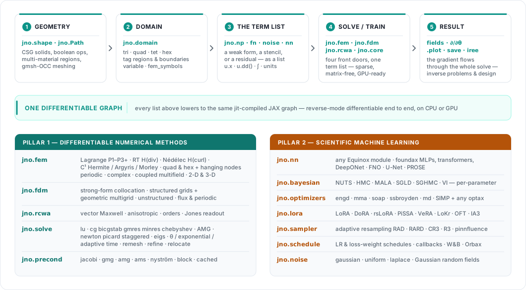
The jNO workflow, and the modules of the two pillars

One term list, weak or strong form

The same boundary-value problem — \(-\Delta u = 1\) on the unit square, \(u = 0\) on the boundary — written twice. Only the form changes; the language does not.

import jno

d = jno.shape.rect(0, 0, 1, 1, size=0.05).domain()
xi, yi, _ = d.variable("interior", split=True)
xb, yb, _ = d.variable("boundary", split=True)

# FEM — the WEAK form is the term list (with a test function v):
u, v = d.fem_symbols()
ui, vi = u.bind(x=xi, y=yi), v.bind(x=xi, y=yi)
u_fem = jno.fem([ui.x * vi.x + ui.y * vi.y - 1.0 * vi,   # ∫∇u·∇v − ∫f·v = 0
                 u(xb, yb) - 0.0]).solve()

# FDM — the STRONG form: the same term list, no test function, collocated at the nodes:
w  = d.unknown()
wi = w.bind(x=xi, y=yi)
u_fdm = jno.fdm([-wi.xx - wi.yy - 1.0,                   # −Δu = 1
                 w(xb, yb) - 0.0]).solve()

Both are sparse, matrix-free, GPU-ready, and end-to-end differentiable — which is what makes the next section possible: wrap either in an objective and the gradient comes back through the solve.

Get started

Install

Pip, Pixi, or Docker — under 30 seconds. CPU out of the box, GPU one extra away.
Getting Started

A 2-D Poisson problem end to end: domain, residual, solve, evaluate.
Tutorials

33 worked examples — PINN, operator learning, FEM, FDM, and Bayesian.
API Reference

Auto-generated from the docstrings: jno.core, jno.domain, jno.np, jno.solve, jno.precond, and more.

What works today

Maturity is stated per capability; each link goes to the page that documents it.

Pillar 1 — Differentiable numerical methods

Capability	Maturity	Notes
FEM, nodal — `jno.fem`	stable	Lagrange P1 / P2 / P3+, 2-D & 3-D; steady (linear + Newton), transient (θ-method), second-order-in-time (wave / elastodynamics), complex, periodic, coupled multifield
FEM, non-nodal — H(div) / H(curl) / C¹	experimental	Raviart–Thomas (H(div)) and Nédélec edge (H(curl) — Maxwell, eddy currents) elements; C¹ Hermite / Argyris / Morley (plates, biharmonic)
Quadrilateral & hexahedral cells	beta	Tensor-product cells with local refinement and hanging nodes
FDM — `jno.fdm`	stable	Strong-form collocation from a term list; structured grids + geometric multigrid; unstructured meshes; periodic, coupled, flux BCs; vector unknowns (Navier–Stokes, elasticity); stencils chosen with `jno.fd(order=, points=, upwind=, fit=, …)`; 2-D & 3-D
Spectral / RCWA — `jno.rcwa`	stable	Vector-Maxwell RCWA, anisotropic media, Jones / polarization readout
Linear & nonlinear solvers — `jno.solve` / `jno.precond`	stable	Sparse-direct LU, Jacobi-BiCGStab, GMRES, CG, MINRES, Chebyshev, geometric multigrid, optional GPU AMG — matrix-free and differentiable
Generalized eigenproblems — `fem.eigs`	beta	`K x = λ M x`, differentiable, M-orthonormal
Time integration	stable	θ-method (backward-Euler / Crank–Nicolson), BDF2, SDIRK, Rosenbrock, exponential integrators, adaptive step size, all through `fem.solve(time=…)`; `jno.fdm` takes the same slot (tested there: θ, BDF2, adaptive; the exponential integrator is refused)
Adaptive & moving meshes	beta	Hessian-metric remeshing (AFEM), r-adaptivity, moving meshes stated in the term list
Differentiable inverse / PDE-constrained	stable	Recover a scalar, a field `k(x)`, the geometry, or a neural coefficient through any solve — the gradient flows through the whole march
Geometry — `jno.shape` / `jno.Path`	stable	CSG via gmsh-OCC; conforming multi-material regions

Pillar 2 — Scientific machine learning

Capability	Maturity	Notes
Forward PINNs (residual minimisation)	stable	Hard or soft BC enforcement
Variational PINNs (weak-form losses)	stable	Network trial functions against the FEM weak form
Operator learning (DeepONet, FNO, U-Net, PROSE via foundax)	stable	PDE-residual or data-driven
Adaptive resampling (RAD, RARD, CR3, R3, pinnfluence)	stable
Stochastic PDEs & noise nodes (gaussian / uniform / laplace)	stable	Fokker–Planck, stochastic forcing
Bayesian PINNs (NUTS, HMC, MALA, SGLD, SGHMC, VI)	stable	`model.bayesian(kernel_factory)` mirrors `.optimizer()` — per-parameter, mixed freely
Parameter-efficient fine-tuning (LoRA, DoRA, rsLoRA, PiSSA, VeRA, LoKr, OFT, IA3)	stable	Chain `.lora(...)` on any wrapped model
Training explainability (gradient conflict, NTK, Hessian, loss landscape, input sensitivity)	stable
Foundation-model integration (foundax MLPs, transformers, DeepONet, FNO, PROSE)	stable	Wrap any Equinox module via `jno.nn(...)`
Hybrid data + model parallelism	stable	`jno.core(..., mesh=(batch, model))`
Hyperparameter / architecture search	beta	Grid + Nevergrad
W&B logging + Orbax checkpointing	stable
IREE / MLIR compiled inference for deployment	stable

Common terminology

A few jNO-specific terms appear throughout the docs. See the Glossary for full definitions:

Trace / tracing system — the unified symbolic graph that holds domain points, network calls, residuals, and losses.
Placeholder — any symbolic node in that graph (a Variable, a network call, an operator).
Constraint — a single optimisable expression passed to jno.core([…]). Typically pde.mse, but can be any scalar.
Term list — the list handed to jno.fem / jno.fdm / jno.rcwa: volume physics, natural boundary terms, and essential BCs, all in one list.
Model controls — fine-grained per-parameter knobs (freeze, LoRA, initialisation, dtype) configured on a wrapped network.
Mesh — overloaded: a spatial mesh for the PDE domain and a device mesh (batch, model) for parallelism.

Tutorials

45 tutorial pages: 43 worked examples and two overviews. Start with the PINN group if you are new to jNO; jump straight to FEM or FDM if you arrived for the solvers.

Group	Count	Covers
PINN	8	Laplace 1-D, variable-coefficient Poisson, Allen–Cahn, viscous Burgers, inverse parameter, Fredholm integral equation, gradient conflict, Fokker–Planck
Operator learning	3	Overview, DeepONet on a parametric Poisson, FNO2D supervised
FEM	27	Poisson, VPINN, Deep Ritz, Helmholtz + PML, elasticity, Navier–Stokes (2-D and 3-D, stabilised, high Re, vortex shedding), droplets, LES subgrid models, laser melt pool, tied two-mesh coating, Rayleigh–Bénard, phase-field fracture, wave & elastodynamics, full-waveform inversion, inverse diffusivity field, adaptive refinement, topology optimisation, 2-D Maxwell
FDM	4	Poisson, heat, mixed BC, inverse source
Bayesian	2	Overview and an inverse coefficient with uncertainty
RCWA	1	Binary-grating diffraction orders

The full list is in the Tutorials tab; the source scripts live under docs/tutorial_examples/.

Cite jNO

Citing helps us justify continued development. See the Cite this repository button on GitHub (reads CITATION.cff) or copy the BibTeX entry from the README. The design is described in arXiv:2605.10159.