Transient Navier–Stokes: the lid-driven cavity (nonlinear flow)

Download .py Back to chapter

The canonical viscous-flow benchmark — and a genuinely nonlinear one. The fluid starts at rest; the top lid is set impulsively in motion and drives a recirculating vortex that spins up to steady state, governed by the incompressible Navier–Stokes equations:

\[\partial_t\mathbf u + (\mathbf u\!\cdot\!\nabla)\mathbf u - \nu\,\Delta\mathbf u + \nabla p = 0,\qquad \nabla\!\cdot\mathbf u = 0,\qquad \mathrm{Re}=\tfrac{UL}{\nu}=200.\]

The convective term is the whole point

(u·∇)u is written inner(grad u, u) — the unknown contracted with itself, a true nonlinearity (unlike the bilinear inner(grad u, grad v), which is trial × test). jno.fem detects this and routes the coupled system to its nonlinear operator, with the Jacobian from autodiff:

conv = inner(gu, ub, n_contract=1)                            # (u·∇)u
momentum = inner(ub.t, vb, n_contract=1) + inner(conv, vb, n_contract=1) \
         + nu*inner(gu, gv, n_contract=2) - pp*trace(gv)
fem = jno.fem([momentum, -qq*trace(gu), ...lid + no-slip + IC...])
assert fem.is_transient and not fem.is_linear                  # transient + nonlinear + coupled

Bring your own implicit stepper (backward Euler + Newton)

fem hands back the semidiscrete pieces as ready-to-use JAX arrays — fem.M (dense mass), fem.state0, and fem.residual(w, t) / fem.jacobian(w, t) (flat residual, dense Jacobian) — so we step it implicitly with a Newton solve per step (the Jacobian is M/Δt + ∂R/∂u), which converges quadratically:

M, w = fem.M, fem.state0                          # dense mass + initial state, ready to use
for step in range(nsteps):                       # backward Euler
    w_prev = w
    for _ in range(8):                            # Newton
        G  = M @ (w - w_prev)/dt + fem.residual(w, t_next)
        dw = jnp.linalg.solve(M/dt + fem.jacobian(w, t_next), -G)
        w  = w + dw

The result

Animation: from a fluid at rest, the moving lid spins up a single large recirculating vortex whose
centre sits above and toward the moving-lid side; two small counter-rotating eddies form in the
bottom corners.

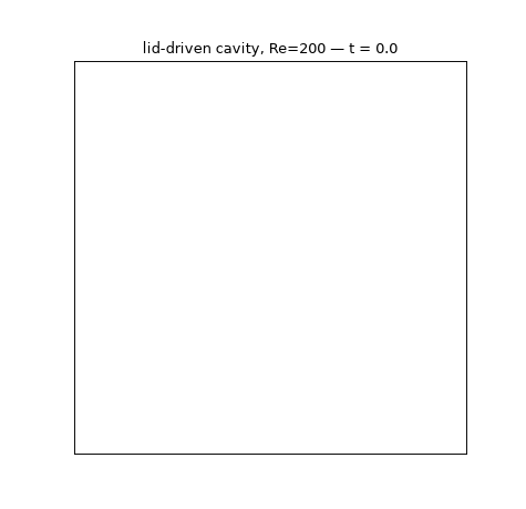
From rest, a primary vortex spins up; at Re=200 its centre sits off-centre (a convective effect — Stokes flow would be symmetric) and two secondary corner eddies appear at the bottom — the textbook cavity structure.

What to notice

Navier–Stokes works now. The convective term used to be silently misclassified as linear; it is detected as nonlinear, so the convection is actually solved (Taylor–Hood P2/P1, autodiff Jacobian). Steady and transient both work.
Bring your own integrator again — here backward Euler + Newton on the block's mass/residual/jacobian. The Newton iteration converges quadratically.
Verified by physics: the flow reaches steady state (the last frames stop changing) and shows a genuine recirculation — the centre-line \(u_x\) is \(+\) near the lid and \(-\) near the floor.

Scope note

This is a closed (lid-driven) flow, so it is all-Dirichlet and needs no outflow boundary. Open flows with vortex shedding (a cylinder in a channel) additionally need a natural outflow boundary — a current jno.fem gap — and, for a developed von Kármán street, long time integration on a fine wake mesh; in 3D that is beyond a single 8 GB GPU. The nonlinear Navier–Stokes machinery shown here is the prerequisite for all of that.

Full script

"""Transient incompressible **Navier-Stokes** in 2D: the lid-driven cavity, the canonical viscous-flow
benchmark. The fluid starts at rest; the top lid is set impulsively in motion and drives a
recirculating vortex that spins up and settles to steady state.

    u_t + (u.grad)u - nu lap u + grad p = 0,    div u = 0,    Re = U L / nu = 200.

The point of this example is the **convective term** ``(u.grad)u`` -- written as ``inner(grad u, u)``.
That is the unknown contracted with itself (a genuine nonlinearity), so ``jno.fem`` routes the whole
system to its nonlinear coupled operator and the Jacobian comes from autodiff. We bring our own
implicit time stepper: **backward Euler + Newton** on the mass / residual / jacobian that ``jno.fem``
exposes for the transient system.

Inf-sup-stable Taylor-Hood elements (P2 velocity, P1 pressure); all-Dirichlet (a regularised moving
lid + no-slip walls), so no outflow boundary is needed.
"""

import os

os.environ["MPLBACKEND"] = "Agg"
os.environ.setdefault("XLA_PYTHON_CLIENT_MEM_FRACTION", "0.6")  # play nice on a shared GPU

import jax

jax.config.update("jax_enable_x64", True)  # the assembler builds in float64

from pathlib import Path  # noqa: E402

import jax.numpy as jnp  # noqa: E402
import matplotlib.animation as animation  # noqa: E402
import matplotlib.pyplot as plt  # noqa: E402
import numpy as np  # noqa: E402
from scipy.interpolate import griddata  # noqa: E402
from shapely.geometry import box  # noqa: E402

import jno  # noqa: E402

inner, grad, trace = jno.np.inner, jno.np.grad, jno.np.trace
nu = 0.005  # Re = U L / nu = 1 * 1 / 0.005 = 200

d = jno.domain(box(0, 0, 1, 1), mesh_size=0.045, time=(0.0, 8.0, 33))
u, v = d.fem_symbols(value_shape=(2,), names=("u", "v"), order=2)  # P2 velocity
p, q = d.fem_symbols(names=("p", "q"), order=1)  # P1 pressure
xi, yi, ti = d.variable("interior", split=True)
xb, yb, _ = d.variable("boundary", split=True)
ci = d.variable("initial", split=True)
ub, vb = u.bind(x=xi, y=yi, t=ti), v.bind(x=xi, y=yi, t=ti)
gu, gv = grad(u, [xi, yi]), grad(v, [xi, yi])
pp, qq = p.bind(x=xi, y=yi, t=ti), q.bind(x=xi, y=yi, t=ti)
conv = inner(gu, ub, n_contract=1)  # (u.grad)u  -- the convective nonlinearity
lid = 16.0 * xb**2 * (1 - xb) ** 2  # regularised lid (peak 1 at x=0.5, 0 at the corners)
momentum = inner(ub.t, vb, n_contract=1) + inner(conv, vb, n_contract=1) + nu * inner(gu, gv, n_contract=2) - pp * trace(gv)
fem = jno.fem(
    [
        momentum,
        -qq * trace(gu),
        u(xb, yb)[0] - jno.np.where(yb > 1 - 1e-6, lid, 0.0),  # moving lid on top, no-slip elsewhere
        u(xb, yb)[1] - 0.0,
        p.pin(),  # gauge-fix: remove the pressure null space (any single DOF)
        u(ci[0], ci[1])[0] - 0.0,  # start from rest
        u(ci[0], ci[1])[1] - 0.0,
    ]
)
assert fem.is_transient and not fem.is_linear, "transient Navier-Stokes must be nonlinear"
off = fem.offsets
M, dt = fem.M, float(fem.dt)
print(f"\nTransient Navier-Stokes lid-driven cavity (Re={1 / nu:.0f}): dofs={fem.dofs}")

# bring-your-own implicit integrator: backward Euler + Newton  ((M/dt + dR/du) du = -G)
nsteps, nframes = round((float(fem.t1) - float(fem.t0)) / dt), 32
w = fem.state0
frames, save_every = [np.asarray(w)], max(1, nsteps // nframes)
for step in range(nsteps):
    w_prev, t_next = w, (step + 1) * dt
    for _ in range(8):  # Newton
        G = M @ (w - w_prev) / dt + fem.residual(w, t_next)
        J = M / dt + fem.jacobian(w, t_next)
        dw = jnp.linalg.solve(J, -G)
        w = w + dw
        if float(jnp.linalg.norm(dw)) < 1e-9:
            break
    if (step + 1) % save_every == 0:
        frames.append(np.asarray(w))
frames = np.stack(frames)
settle = float(np.linalg.norm(frames[-1] - frames[-2]) / np.linalg.norm(frames[-1]))

pts_v = np.asarray(fem.field_points[0])
vel = frames[:, off[0] : off[1]].reshape(frames.shape[0], -1, 2)  # (frame, n_vel_nodes, 2)
uxN = vel[-1, :, 0]  # steady x-velocity, for the recirculation check
cl = np.abs(pts_v[:, 0] - 0.5) < 0.06  # near the vertical centre-line
top = uxN[cl & (pts_v[:, 1] > 0.7)].mean()  # driven by the lid -> u_x > 0
bot = uxN[cl & (pts_v[:, 1] < 0.3)].mean()  # return flow -> u_x < 0
print(f"  steady by final frame: {settle:.3e}  |  centre-line u_x  top={top:+.3f}  bottom={bot:+.3f} (recirculation)")

# ---- animate the spinning-up vortex: streamlines coloured by speed -> a GIF ----
gx, gy = np.meshgrid(np.linspace(0, 1, 90), np.linspace(0, 1, 90))
fig, ax = plt.subplots(figsize=(5.6, 5.4))


def _frame(j):
    ax.clear()
    UX = griddata(pts_v, vel[j, :, 0], (gx, gy), method="linear")
    UY = griddata(pts_v, vel[j, :, 1], (gx, gy), method="linear")
    ax.streamplot(gx, gy, UX, UY, color=np.hypot(UX, UY), cmap="viridis", density=1.4, linewidth=0.8)
    ax.set_aspect("equal")
    ax.set_xlim(0, 1)
    ax.set_ylim(0, 1)
    ax.set_xticks([])
    ax.set_yticks([])
    ax.set_title(f"lid-driven cavity, Re=200 — t = {j * save_every * dt:.1f}", fontsize=11)


ani = animation.FuncAnimation(fig, _frame, frames=vel.shape[0], interval=110, blit=False)
ani.save(Path(__file__).parents[2] / "assets" / "navier_stokes_cavity_2d.gif", writer="pillow", fps=9, dpi=85)

assert settle < 2e-2, f"flow not at steady state by the final frame: {settle:.3e}"
assert top > 0.1 and bot < -0.02, f"expected a recirculating vortex (u_x top>0, bottom<0): top={top:.3f} bot={bot:.3f}"