Vibrating Membrane (2-D wave, second order in time)

Download .py All tutorials

A square drum head, clamped on all four edges, plucked into its fundamental mode and released: \(u_{tt}=c^2\Delta u\) with \(u=0\) on the boundary. This is the first second-order-in-time FEM problem — the unknown carries a second time derivative ui.tt, which jno.fem auto-reduces to a first-order system in \(y=[u,\,v{=}u_t]\).

A second time derivative + two initial conditions

ui.tt makes the form second order; a second-order problem needs two initial conditions — displacement and velocity. The velocity IC binds the "initial"-slice coordinates and time ti0 (the .t derivative carries its region on the temporal variable):

xi0, yi0, ti0 = d.variable("initial", split=True)
ui0 = u.bind(x=xi0, y=yi0, t=ti0)
weak = ui.tt * vi + C**2 * (ui.x * vi.x + ui.y * vi.y)      # ∫ u_tt φ + c² ∫ ∇u·∇φ = 0
fem  = jno.fem([weak, u(xb, yb) - 0.0,
                u(xi0, yi0) - jno.fn(pluck, [xi0, yi0]),    # displacement IC
                ui0.t - 0.0])                               # velocity IC (at rest)

fem.solve() steps with θ=½, not backward Euler

The augmented block has state \(y=[u;v]\) of size \(2N\) — split with fem.offsets ([0, N, 2N]). fem.solve() integrates it itself with the energy-conserving trapezoidal rule (θ=½) — not plain backward Euler, which (unlike the parabolic first-order case) would spuriously damp an undamped membrane. For a transient solve the result is a differentiable trace node, so we read the trajectory (one \(y\) per step) through a minimal crux and split it into displacement and velocity:

N   = fem.offsets[1]                                 # y = [u; v]; first N = displacement
sol = fem.solve()                                    # θ=½ trapezoidal stepping, done inside
state = np.asarray(jno.core([sol.mse]).eval([sol]))  # (n_steps, 2N) trajectory of y = [u; v]
traj, V = state[:, :N], state[:, N:]                 # displacement and velocity histories

The energy check \(E=\tfrac12 v^\top M v+\tfrac12 u^\top K u\) still pulls the mass/stiffness blocks straight from fem.M and fem.operator.A.

What to notice

• ui.tt triggers the second-order route; ui.t is the velocity. The state is y = [u; v].
• The centre antinode tracks the analytic standing wave \(\sin(\pi x)\sin(\pi y)\cos(\omega t)\), \(\omega=c\pi\sqrt2\), to ~1% over a full period.
• The amplitude after one period is conserved (\(\approx 1\)) — the trapezoidal rule does not bleed energy from an undamped wave (Newmark average-acceleration; Newmark 1959).

Result

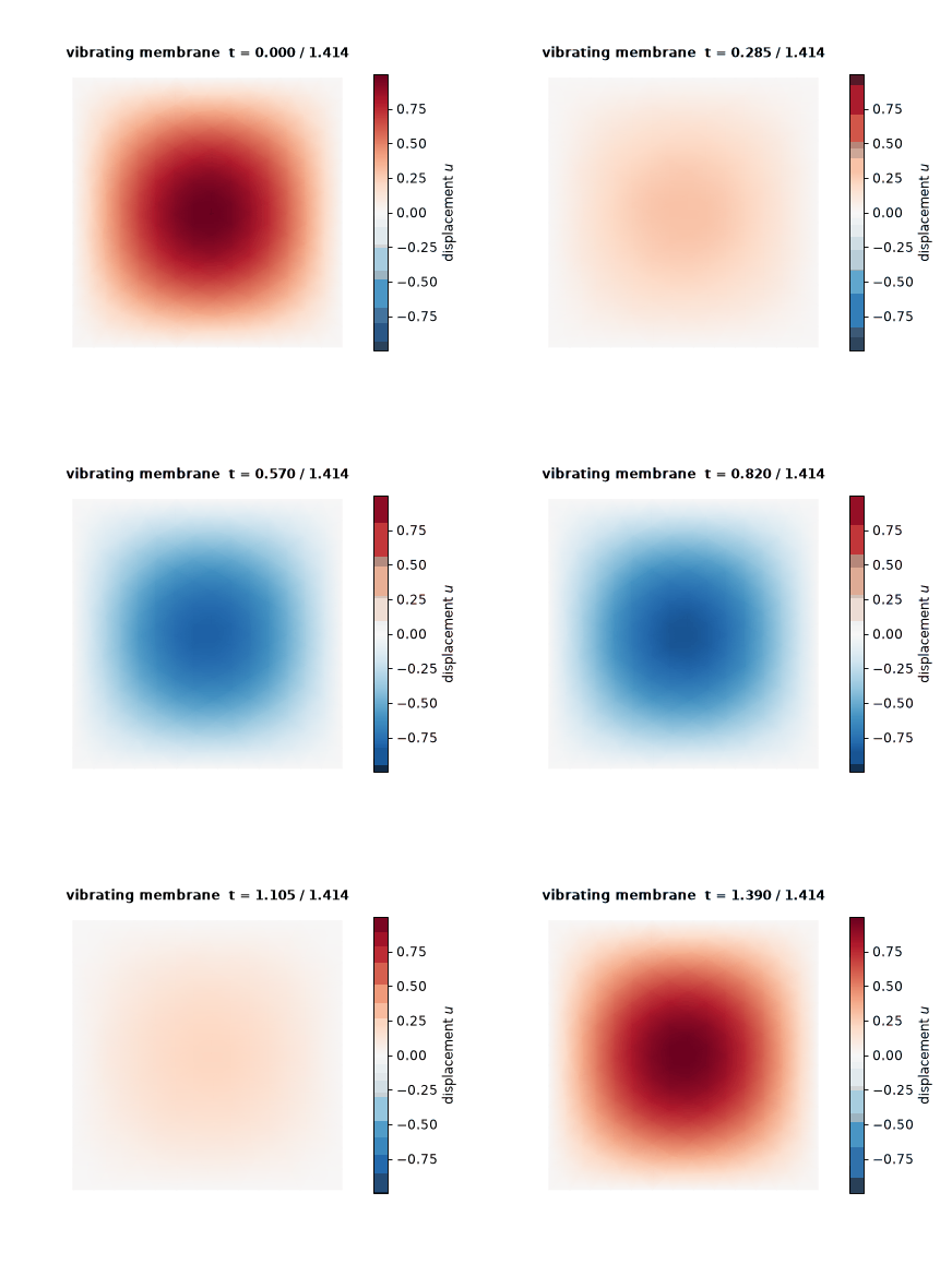
The fundamental mode swings between its positive and negative extremes and back over one period, on a colour scale held fixed and symmetric across every frame.

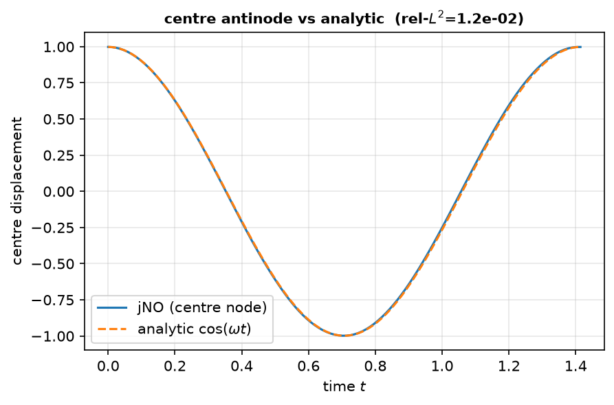
The centre antinode tracks the analytic standing wave \(\sin(\pi x)\sin(\pi y)\cos(\omega t)\) to rel-\(L^2\approx1.2\times10^{-2}\) over the full period, and the amplitude is conserved (\(\approx1\)) — the trapezoidal (\(\theta=\tfrac12\)) rule does not bleed energy from the undamped drum.

Full script

"""09 - Vibrating membrane: the 2-D wave equation (second-order in time) via ``jno.fem``.

A square drum head clamped on all four edges, plucked into the fundamental mode and released:

    u_tt = c^2 Δu ,    u = 0 on ∂Ω ,    u(t=0) = sin(πx) sin(πy) ,   u_t(t=0) = 0 .

The exact solution is the standing wave  u(x, y, t) = sin(πx) sin(πy) cos(ω t)  with the modal
frequency  ω = c π √2  (so  -Δ(sin πx sin πy) = 2π² · sin πx sin πy).  This is a **second-order**
weak form -- the unknown carries a *second* time derivative ``ui.tt`` -- which ``jno.fem`` auto-reduces
to the first-order system in y = [u, v=u_t] and exposes as the usual transient block ``fem.M`` /
``fem.operator.A`` / ``fem.state0``.

Time integration uses the **trapezoidal rule** (θ=½, the energy-conserving member of the Newmark
average-acceleration family -- Newmark 1959, *J. Eng. Mech. Div. ASCE* 85(3)). For a *second-order*
block this matters: backward Euler would spuriously damp an undamped membrane, so we step with θ=½
rather than the backward-Euler pattern used for parabolic (first-order) problems.

Verification: the centre-node displacement tracks the analytic cos(ω t) over a full period, and the
discrete energy E = ½ vᵀM v + ½ uᵀK u is conserved (a drum does not lose energy on its own).
"""

import jax.numpy as jnp
import numpy as np

import jno

dense = lambda A: jnp.asarray(A.todense()) if hasattr(A, "todense") else jnp.asarray(A)  # noqa: E731

PI = np.pi
C = 1.0  # wave speed
OMEGA = C * PI * np.sqrt(2.0)  # fundamental modal frequency
PERIOD = 2.0 * PI / OMEGA  # = √2 / C

# One full period, resolved with 120 steps; a moderate mesh keeps the example quick.
d = jno.Shape.rect(0.0, 0.0, 1.0, 1.0, size=0.08).domain(time=(0.0, float(PERIOD), 120))
u, phi = d.fem_symbols()
xi, yi, ti = d.variable("interior", split=True)
xb, yb, _ = d.variable("boundary", split=True)
xi0, yi0, ti0 = d.variable("initial", split=True)  # the t=0 slice carries its coords AND time ti0
ui, vi = u.bind(x=xi, y=yi, t=ti), phi.bind(x=xi, y=yi, t=ti)
ui0 = u.bind(x=xi0, y=yi0, t=ti0)

# Weak form of u_tt = c² Δu :  ∫ u_tt φ + c² ∫ ∇u·∇φ = 0 .
weak = ui.tt * vi + C**2 * (ui.x * vi.x + ui.y * vi.y)
u0 = u(xi0, yi0) - jno.fn(lambda x, y: jnp.sin(PI * x) * jnp.sin(PI * y), [xi0, yi0])  # plucked shape
v0 = ui0.t - 0.0  # released from rest (note: velocity IC binds the initial-slice time ti0)
fem = jno.fem([weak, u(xb, yb) - 0.0, u0, v0])
assert fem.is_transient and fem.is_linear

# --- solve: fem.solve() integrates the augmented block with the energy-conserving
#     trapezoidal (θ=½) rule *internally* -- no hand-rolled time stepping. (Backward Euler would
#     damp the wave; that is why the transient solver uses θ=½ for a second-order block.)
#     fem.solve() is a differentiable trace node; evaluate the forward trajectory through a crux.
N = fem.offsets[1]  # state is y = [u; v]; displacement is the first N entries, velocity the last N
sol = fem.solve()
state = np.asarray(jno.core([sol.mse]).eval([sol]))  # (n_steps, 2N) trajectory of y = [u; v]
traj, V = state[:, :N], state[:, N:]  # displacement and velocity histories (v = u_t, exact)
ts = np.linspace(fem.t0, fem.t1, traj.shape[0])

# --- verify against the analytic standing wave + energy conservation ---
pts = np.asarray(fem.points)
ci = int(np.argmin(np.sum((pts - 0.5) ** 2, axis=1)))  # node nearest the centre antinode
u_center = traj[:, ci]
u_exact = np.sin(PI * pts[ci, 0]) * np.sin(PI * pts[ci, 1]) * np.cos(OMEGA * ts)
rel = np.linalg.norm(u_center - u_exact) / np.linalg.norm(u_exact)

M_full, A_full = dense(fem.M), dense(fem.operator.A)
M_uu, K_uu = M_full[:N, :N], A_full[N:, :N]  # mass and stiffness blocks of the augmented system
energy = 0.5 * np.einsum("ti,ij,tj->t", V, M_uu, V) + 0.5 * np.einsum("ti,ij,tj->t", traj, K_uu, traj)
amp = np.linalg.norm(traj[-1]) / np.linalg.norm(traj[0])

print(f"\nVibrating membrane (2-D wave, second-order in time): dofs={fem.dofs} (= 2N, N={N})")
print(f"  modal frequency ω = c·π·√2 = {OMEGA:.4f}   period T = {PERIOD:.4f}")
print(f"  centre-node vs analytic cos(ω t) over one period:  rel L2 = {rel:.4f}")
print(f"  amplitude after one period ||u(T)|| / ||u(0)|| = {amp:.4f}   (≈ 1: energy-conserving)")

assert rel < 0.05, f"membrane does not track the analytic standing wave: rel L2 = {rel:.4f}"
assert 0.95 < amp < 1.05, f"amplitude not conserved over a period: {amp:.4f}"  # θ=½, not backward Euler
assert abs(energy[len(energy) // 2] / energy[1] - 1.0) < 0.05, "discrete energy should be conserved"