Transient Heat 2D (FDM)

Download .py All tutorials

The heat equation \(u_t = \nu\,\Delta u\) on the unit square with \(u = 0\) on the boundary and \(u_0 = \sin(\pi x)\sin(\pi y)\), whose exact solution decays as \(u = e^{-2\nu\pi^2 t}\sin(\pi x)\sin(\pi y)\). Solved through jno.fdm by the method of lines.

Result

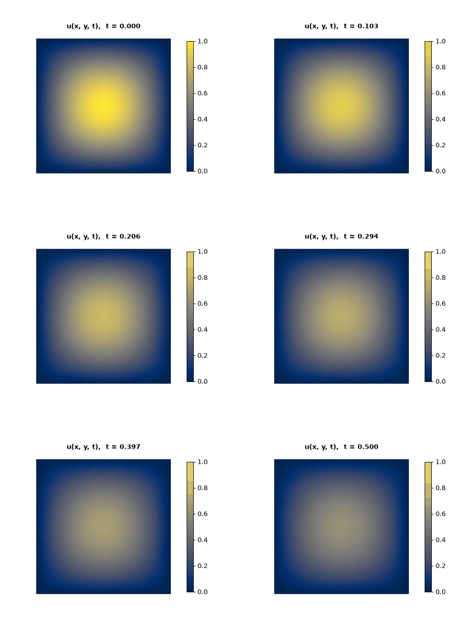
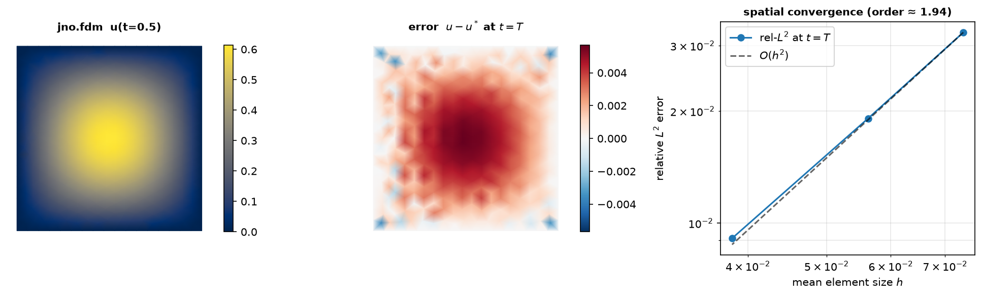
The initial \(\sin(\pi x)\sin(\pi y)\) bump decays smoothly under the method-of-lines march (peak \(1 \to \approx 0.61\) by \(t = 0.5\)). At the final time the field matches the analytic decay to rel-\(L^2 \approx 9.1\times10^{-3}\), and re-solving at three mesh sizes (200 steps each) shows the spatial error falling at second order (fitted slope \(\approx 1.94\), right).

The initial condition is a constraint

As in jno.fem, a problem is transient exactly when it carries an initial condition — and the IC is found from the constraints (u(xi, yi) - u0, with xi, yi the "initial" region), never a config flag. The time window and step count come from domain.time = (t0, t1, n), and the u.t term marks the time derivative:

d = jno.Shape.rect(0, 0, 1, 1, size=0.06).domain(time=(0.0, 0.5, 200))
x, y, t   = d.variable("interior", split=True)     # temporal Variable t
xi, yi, _ = d.variable("initial",  split=True)     # the t = t0 slice
ui = u.bind(x=x, y=y, t=t)

traj = jno.fdm([
    ui.t - nu * (ui.d2(x) + ui.d2(y)),                 # u_t = nu * Delta u
    u(xb, yb) - 0.0,                                   # Dirichlet
    u(xi, yi) - jnn.sin(np.pi*xi) * jnn.sin(np.pi*yi), # initial condition
]).solve()

What to notice

• .solve() marches by the method of lines, reusing the same semidiscrete time-stepper jno.fem uses — no new time-integration code — and returns the trajectory (n_steps, N).
• t_span and the number of steps are inferred from domain.time; the IC supplies the initial state.
• The final field is audited against the analytic decay (rel-\(L^2 \approx 9\times10^{-3}\) at \(t = 0.5\)).

Full script

"""03 - Transient heat equation through ``jno.fdm`` (method of lines).

    u_t = nu * Delta u  on the unit square,  u = 0 on the boundary,
    u0(x, y) = sin(pi x) sin(pi y)   ->   u(x, y, t) = e^{-2 nu pi^2 t} sin(pi x) sin(pi y).

A problem is **transient** exactly when it carries an initial condition -- and, as in ``jno.fem``,
the IC is *found from the constraints* (``u(xi, yi) - u0``, with ``xi, yi`` the ``"initial"`` region),
never passed as a config flag. The time window and step count come from ``domain.time = (t0, t1, n)``.
The ``u.t`` term marks the time derivative; ``jno.fdm`` marches by the method of lines, reusing the
same semidiscrete time-stepper ``jno.fem`` uses. ``.solve()`` returns the trajectory ``(n_steps, N)``.
"""

import jax

jax.config.update("jax_enable_x64", True)

import numpy as np  # noqa: E402

import jno  # noqa: E402
import jno.jnp_ops as jnn  # noqa: E402

nu, T = 0.05, 0.5
d = jno.Shape.rect(0.0, 0.0, 1.0, 1.0, size=0.06).domain(time=(0.0, T, 200))
x, y, t = d.variable("interior", split=True)  # note the temporal Variable t
xb, yb, _ = d.variable("boundary", split=True)
xi, yi, _ = d.variable("initial", split=True)  # the t = t0 slice
u = d.unknown()
ui = u.bind(x=x, y=y, t=t)

traj = jno.fdm(
    [
        ui.t - nu * (ui.d2(x) + ui.d2(y)),  # u_t = nu * Delta u
        u(xb, yb) - 0.0,  # Dirichlet u = 0
        u(xi, yi) - jnn.sin(np.pi * xi) * jnn.sin(np.pi * yi),  # initial condition u0
    ]
).solve()

p = np.asarray(d.mesh_connectivity["points"])[:, :2]
exact = np.exp(-2 * nu * np.pi**2 * T) * np.sin(np.pi * p[:, 0]) * np.sin(np.pi * p[:, 1])
rel_l2 = float(np.linalg.norm(np.asarray(traj)[-1] - exact) / np.linalg.norm(exact))
print(f"\nTransient heat via jno.fdm: steps=200  rel_L2(t={T})={rel_l2:.3e}")
assert rel_l2 < 2e-2, f"relative L2 error too large: {rel_l2:.3e}"