Deep Ritz: solve a PDE by minimising an energy functional

Download .py All tutorials

A VPINN (previous tutorial) minimises the weak residual test-projected onto the FE basis. The Deep Ritz method takes the other classical route: it minimises the energy functional directly — the network is the trial, there are no test functions and no assembled system. For Poisson \(-\Delta u = f\) with \(u=0\) on \(\partial\Omega\) the governing energy is

\[ J[u] = \int_\Omega \Big( \tfrac12\,|\nabla u|^2 - f\,u \Big)\,dx, \]

whose minimiser over \(H^1_0\) is the weak solution. Lower derivative order (only \(\nabla u\), no \(\Delta u\)) and no linear solve, at the price of a non-convex optimisation.

Method: Deep Ritz — E & Yu, Commun. Math. Stat. 6:1 (2018), §2 (arXiv:1710.00211); the solid-mechanics form is the Deep Energy Method (Samaniego et al., CMAME 362, 2020; Nguyen-Thanh, Zhuang & Rabczuk, Eur. J. Mech. A/Solids 80, 2020).

The energy as a loss

expr.integrate() integrates a scalar expression over the mesh (auto-detecting volume vs boundary from the coordinate variable), so the whole method is: build the network trial, write the energy density, integrate it, and hand the single scalar to jno.core as the loss.

xi, yi, _ = dom.variable("interior", split=True)
net = jnn.nn.wrap(foundax.mlp(2, hidden_dims=48, num_layers=4, activation=jax.nn.tanh, key=key))

ansatz = xi * (1 - xi) * yi * (1 - yi)      # hard-BC ansatz: vanishes on ∂Ω  → u ∈ H¹₀
u  = net(xi, yi) * ansatz
ux, uy = jnn.grad(u, xi), jnn.grad(u, yi)
f  = 2.0 * (xi * (1 - xi) + yi * (1 - yi))

energy = (0.5 * (ux**2 + uy**2) - f * u).integrate(quadrature="gauss")   # J[u] = ∫ (½|∇u|² − f u) dx

net.optimizer(optax.adam(3e-3))
jno.core([energy], domain=dom).solve(4000)             # minimise the (signed) energy directly

The loss is the signed energy — .integrate() reduces to a scalar and jno.core minimises it as is (no square), so the reported loss converges to \(J_{\min}<0\). General geometries that cannot use a hard-BC ansatz add a boundary penalty (β * (net(xb, yb) - g)).mse as a second constraint.

Quadrature consistency — why quadrature="gauss"

The default .integrate() uses the P1 nodal-volume (vertex) rule: the energy is sampled only at the mesh nodes. A network expressive enough to develop structure between nodes can drive the quadrature-estimated energy below the true minimum — a variational crime in which the discrete energy stops being a faithful estimate, and the solution degrades even as the reported loss keeps falling. .integrate(quadrature="gauss") samples the per-element Gauss points (weighting by \(J\,W\)) instead — many points inside each element, far harder to alias — so a capable network can minimise the energy safely. Pass quadrature=<int> to set the Gauss degree ("gauss" = 4).

With this same 48×4 network the two rules diverge sharply: Gauss holds the true minimum and reaches rel-\(L^2 \approx 8\times10^{-5}\), while the nodal rule lets the energy sink past the true minimum and the error blows up. (Gauss integration is currently volume-only; boundary integrals use the nodal rule.)

The result

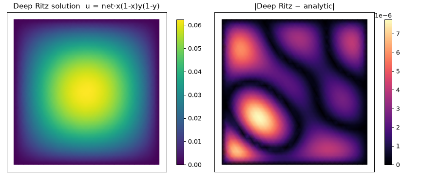
The trained network matches the analytic \(x(1-x)y(1-y)\) to rel-\(L^2 \approx 8\times10^{-5}\). The energy plateaus at the true minimum within a few hundred epochs and stays there.

What to notice

• Energy, not residual. The loss is the functional \(J[u]\) itself, integrated over the mesh with .integrate() — no test functions, no assembled operator. Contrast the VPINN, which needs the FE test space.
• Signed objective. jno.core minimises the raw reduced value, so a signed energy that goes negative is exactly right — no .mse wrapper.
• Quadrature matters for energy losses. A fixed nodal rule can be aliased by an expressive integrand; quadrature="gauss" samples inside each element and resists it. If a loss dips below the analytic energy while the error grows, that is the quadrature being exploited.