Two droplets merge: a diffuse-interface flow (Cahn–Hilliard–Navier–Stokes)
Two liquid drops sit side by side, their rims 0.08 apart. Surface tension pulls them together; they touch, fuse into one, and the merged drop relaxes toward a circle. That is a change of topology — two boundaries become one — and it needs no special machinery here, because the interface is not a mesh boundary at all. It is a field.
A phase field \(\phi\) is \(+1\) in the liquid and \(-1\) outside, with a \(\tanh\) layer of width \(\sim\varepsilon\) between. It rides beside the flow (Jacqmin 1999; Yue, Feng, Liu & Shen 2004):
The chemical potential \(\mu\) is the variational derivative of the interface energy, and \(\mu\nabla\phi\) is the capillary force it exerts on the fluid.
The model is the term list
Nothing in jNO is specific to two-phase flow. The four fields are ordinary FEM symbols — a Taylor–Hood velocity/pressure pair, and P1 fields for \(\phi\) and \(\mu\) — and each equation is a weak form:
momentum = (RHO * dot(u_.t, v_) + RHO * dot(dot(grad_u, u_), v_) + ETA * ddot(grad_u, grad_v)
            - p_ * trace(grad_v) - mu * (phi.x * v_[0] + phi.y * v_[1]))          # capillary force μ∇φ
cahn_hilliard = phi.t * psi + (u_[0] * phi.x + u_[1] * phi.y) * psi + MOBILITY * (mu.x * psi.x + mu.y * psi.y)
chemical_potential = mu * chi - LAM * (phi * phi * phi - phi) / EPS**2 * chi - LAM * (phi.x * chi.x + phi.y * chi.y)
The fourth-order Cahn–Hilliard operator is split into two second-order equations through \(\mu\), so plain \(H^1\) elements carry it.
A mesh that follows the interface
The interface is where the resolution matters, and it moves. remesh(criterion=...) refines on any
traced field — here \(1-\phi^2\), which is \(\approx 1\) on the interface and \(\approx 0\) in both bulks — and on a
march it is evaluated on the live state at every remesh, at a fixed DOF budget (max_dofs counts
every unknown of the system, fem.dofs, not vertices):
phi_now = c.bind(x=xi, y=yi)
traj = fem.solve(adapt=jno.solve.remesh(criterion=1.0 - phi_now * phi_now, every=3, max_dofs=fem.dofs),
                 nonlinear=jno.solve.newton(direct=True))
The starting mesh is already graded toward the two rims (size= takes a callable). Remeshing moves
resolution to where a feature is going; it cannot recover what a coarse first step already lost.
What it produces
8,636 DOFs on 798 vertices, 12 steps, three remeshes — 57 s on this machine (GPU).
| start | end | |
|---|---|---|
| \(\phi\) midway between the drops | \(-0.185\) | \(+1.035\) (one drop) |
| width / height of the liquid | 2.28 | 0.99 (a circle) |
| liquid area \(\int(1+\phi)/2\) | 0.22006 | 0.22185 (+0.81 %) |
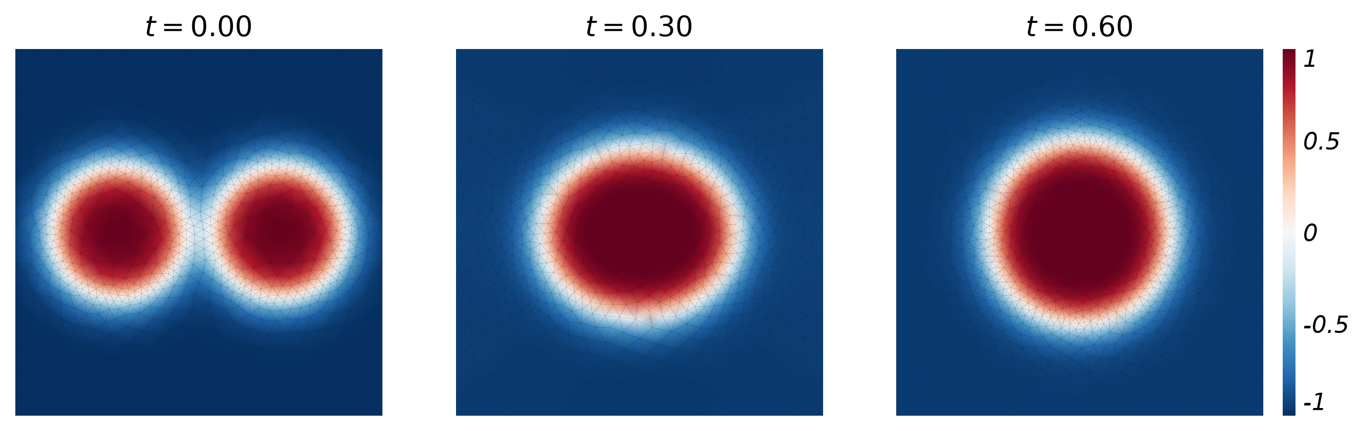
The computed \(\phi\) at \(t = 0\), \(0.30\) and \(0.60\), each drawn on the adapted mesh that step ran on — the fine band tracks the interface as the drops fuse. The colour saturates at \(\pm1\); the bulk itself sits at \(\pm1.03\), the known Cahn–Hilliard shift for a curved interface.
Conservation, stated exactly
Cahn–Hilliard conserves \(\int\phi\) exactly on a fixed mesh: summing the \(\phi\) equation over the P1 partition of unity leaves only \(\int\phi\,\nabla\!\cdot\mathbf u\), and \(\phi\) lies in the P1 pressure-test space, so the discrete continuity equation makes that term vanish. The script asserts it — between remeshes the liquid area is constant to \(10^{-8}\). The +0.81 % over the whole run is therefore entirely the three state transfers, not the model.
The same model passes two static checks in tests/test_fem_chns_droplet.py. A single drop carries the
Laplace pressure jump \(\sigma/R\) to +4.0 % at \(\varepsilon/R = 0.12\) — an \(O(\varepsilon/R)\)
diffuse-interface error that shrinks with \(\varepsilon\) — and its chemical potential settles at the
Gibbs–Thomson value \(\sigma/2R\) to +4.3 %, while the spurious currents die away to \(3\times10^{-6}\) of the
capillary velocity \(\sigma/\eta\).
Scope — what this is not
- Planar 2-D. A planar liquid thread cannot pinch off, so breakup needs an axisymmetric or 3-D run.
- Matched density and viscosity. A density ratio enters through \(\rho(\phi)\) as a state-dependent mass (it assembles, and a static drop at ratio 1000 stays static), but large-ratio dynamics are not checked here.
- A diffuse interface. \(\varepsilon/R = 0.22\) in this run; results carry an \(O(\varepsilon/R)\) error, and a drop slowly shrinks by the Cahn–Hilliard bulk shift. The rims start about 1.4 interface widths apart, so the first contact is helped by diffusion across the gap, not by flow alone.
"""Two droplets **merge** -- a change of topology -- in a Cahn–Hilliard–Navier–Stokes (diffuse-interface)
model, on a mesh that follows the interface. Nothing here is a two-phase feature: the model is the term list.

    rho (u_t + (u.grad)u) = -grad p + eta lap u + mu grad(phi),        div u = 0
    phi_t + u.grad(phi)   = div(M grad mu),       mu = lam (-lap phi + (phi^3 - phi) / eps^2)

phi = +1 in the liquid and -1 outside, and the interface is a tanh layer of width ~eps. Surface tension is
sigma = (2 sqrt2 / 3) lam / eps (Jacqmin 1999; Yue, Feng, Liu & Shen 2004). Because the interface is a
field rather than a boundary, two drops can touch and fuse with no remeshing surgery at all -- and the
mesh is free to follow it, refined where 1 - phi^2 is large and coarse in the bulk.
"""

import os

os.environ.setdefault("XLA_PYTHON_CLIENT_MEM_FRACTION", "0.6")

import jax

jax.config.update("jax_enable_x64", True)

import numpy as np  # noqa: E402

import jno  # noqa: E402

inner, grad, trace = jno.np.inner, jno.np.grad, jno.np.trace
tanh, sqrt = jno.np.tanh, jno.np.sqrt
dot = lambda a, b: inner(a, b, n_contract=1)  # noqa: E731  a·b
ddot = lambda a, b: inner(a, b, n_contract=2)  # noqa: E731  A:B

SIGMA, ETA, RHO = 1.0, 0.1, 1.0  # surface tension, viscosity, density
EPS, MOBILITY = 0.04, 1e-2  # interface width, Cahn–Hilliard mobility
LAM = 3.0 * SIGMA * EPS / (2.0 * np.sqrt(2.0))
R, CX1, CX2, CY = 0.18, 0.28, 0.72, 0.5  # two drops whose rims are 0.08 (~1.4 interface widths) apart
T_END, N_STEPS = 0.6, 12


def near_the_rims(x, y, z):  # gmsh calls a size field with THREE coordinates, in 2-D as well
    rim = min(abs(np.hypot(x - CX1, y - CY) - R), abs(np.hypot(x - CX2, y - CY) - R))
    return 0.02 + 0.04 * min(1.0, rim / 0.12)  # 0.02 at the interfaces, 0.06 in the bulk


d = jno.shape.rect(0, 0, 1, 1, size=near_the_rims).domain(time=(0.0, T_END, N_STEPS + 1))
u, v = d.fem_symbols(value_shape=(2,), names=("u", "v"), order=2)  # P2 velocity
p, q = d.fem_symbols(names=("p", "q"), order=1)  # P1 pressure
c, s = d.fem_symbols(names=("phi", "psi"), order=1)  # P1 phase field
m, w = d.fem_symbols(names=("mu", "chi"), order=1)  # P1 chemical potential
xi, yi, ti = d.variable("interior", split=True)
xb, yb, _ = d.variable("boundary", split=True)
x0, y0, _ = d.variable("initial", split=True)
B = dict(x=xi, y=yi, t=ti)
u_, v_, p_, q_ = u.bind(**B), v.bind(**B), p.bind(**B), q.bind(**B)
phi, psi, mu, chi = c.bind(**B), s.bind(**B), m.bind(**B), w.bind(**B)
grad_u, grad_v = grad(u, [xi, yi]), grad(v, [xi, yi])

momentum = (
    RHO * dot(u_.t, v_)
    + RHO * dot(dot(grad_u, u_), v_)
    + ETA * ddot(grad_u, grad_v)
    - p_ * trace(grad_v)
    - mu * (phi.x * v_[0] + phi.y * v_[1])  # the capillary force  mu grad(phi)
)
continuity = -q_ * trace(grad_u)
cahn_hilliard = phi.t * psi + (u_[0] * phi.x + u_[1] * phi.y) * psi + MOBILITY * (mu.x * psi.x + mu.y * psi.y)
chemical_potential = mu * chi - LAM * (phi * phi * phi - phi) / EPS**2 * chi - LAM * (phi.x * chi.x + phi.y * chi.y)


def drop(cx):
    return tanh((R - sqrt((x0 - cx) ** 2 + (y0 - CY) ** 2)) / (np.sqrt(2.0) * EPS))


fem = jno.fem(
    [
        momentum,
        continuity,
        cahn_hilliard,
        chemical_potential,
        u(xb, yb)[0] - 0.0,  # no-slip walls
        u(xb, yb)[1] - 0.0,
        p.pin(),  # the pressure is defined up to a constant
        u(x0, y0)[0] - 0.0,  # start at rest
        u(x0, y0)[1] - 0.0,
        c(x0, y0) - (drop(CX1) + drop(CX2) + 1.0),  # two drops
    ]
)
n0 = int(np.asarray(d.mesh.points).shape[0])
print(f"CHNS droplet merger: {fem.dofs} DOFs on {n0} vertices")

phi_now = c.bind(x=xi, y=yi)
traj = fem.solve(
    adapt=jno.solve.remesh(criterion=1.0 - phi_now * phi_now, every=3, max_dofs=fem.dofs),  # follow the interface
    nonlinear=jno.solve.newton(direct=True),  # a sparse-direct Newton per step: the saddle needs it
)
ic = fem.block_index(c)  # which block of the state is phi


def phase(k):
    """phi on its own nodes at frame k, and int (1 + phi)/2 -- the liquid area -- by the P1 vertex rule."""
    lay = traj.layouts[k]
    pts = np.asarray(lay["field_points"][ic])[:, :2]
    val = np.asarray(traj.states[k])[lay["offsets"][ic] : lay["offsets"][ic + 1]]
    tri = np.asarray(lay["cells_f"][ic])[:, :3]
    P = pts[tri]
    area = 0.5 * np.abs(
        (P[:, 1, 0] - P[:, 0, 0]) * (P[:, 2, 1] - P[:, 0, 1]) - (P[:, 2, 0] - P[:, 0, 0]) * (P[:, 1, 1] - P[:, 0, 1])
    )
    return pts, val, float(np.sum(area * (1.0 + val[tri]).mean(axis=1) / 2.0))


def gap(pts, val):  # phi midway between the two drops
    return float(val[np.argmin(np.hypot(pts[:, 0] - 0.5, pts[:, 1] - CY))])


def aspect(pts, val):  # width / height of the liquid region
    liquid = pts[val > 0.0]
    return float(np.ptp(liquid[:, 0]) / np.ptp(liquid[:, 1]))


areas = [phase(k)[2] for k in range(len(traj))]
pts0, phi0, liquid0 = phase(0)
ptsN, phiN, liquidN = phase(len(traj) - 1)
remeshes = sum(bool(h.get("remeshed")) for h in fem.adapt_history)
# Cahn–Hilliard conserves int phi EXACTLY on a fixed mesh -- so between two remeshes (frames that share one
# mesh) the liquid area is constant to solver precision, and any drift is the state transfer at a remesh.
same_mesh = [k for k in range(len(traj) - 1) if traj.meshes[k] is traj.meshes[k + 1]]
between = max(abs(areas[k + 1] - areas[k]) for k in same_mesh)
print(f"  gap phi: {gap(pts0, phi0):+.3f} -> {gap(ptsN, phiN):+.3f}   (two drops -> one)")
print(f"  width/height: {aspect(pts0, phi0):.2f} -> {aspect(ptsN, phiN):.2f}   (relaxing toward a circle)")
print(f"  liquid area: {liquid0:.5f} -> {liquidN:.5f}  ({(liquidN / liquid0 - 1) * 100:+.2f} %, over {remeshes} remeshes)")
print(f"  largest change between remeshes: {between:.1e}")

assert gap(pts0, phi0) < 0.0 < 0.9 < gap(ptsN, phiN), "the two drops did not merge"
assert aspect(ptsN, phiN) < 0.8 * aspect(pts0, phi0), "the merged drop is not relaxing toward a circle"
assert between < 1e-8, f"int phi changed by {between:.1e} on a fixed mesh -- Cahn–Hilliard conserves it exactly"
assert abs(liquidN / liquid0 - 1.0) < 2e-2, (
    "the remesh transfers lost or gained more liquid than expected"
)  # measured +0.81 %
assert remeshes >= 2, "the mesh never followed the interface"
References. D. Jacqmin, J. Comput. Phys. 155 (1999) 96–127. P. Yue, J. J. Feng, C. Liu & J. Shen, J. Fluid Mech. 515 (2004) 293–317.