DFG 2D-2: vortex shedding at Re = 100
The 2D-1 tutorial solves the steady cylinder at Re = 20. Drive it
three times harder and the wake goes unstable: a von Kármán street, shedding at a frequency the
benchmark publishes. This is the external check on the stabilised-flow work — it exercises the vector
Laplacian, dom.cell_metric and jno.solve.bdf2() in one run, against a number nobody in this repo
chose.
Configuration is Schäfer & Turek (1996), benchmark 2D-2.
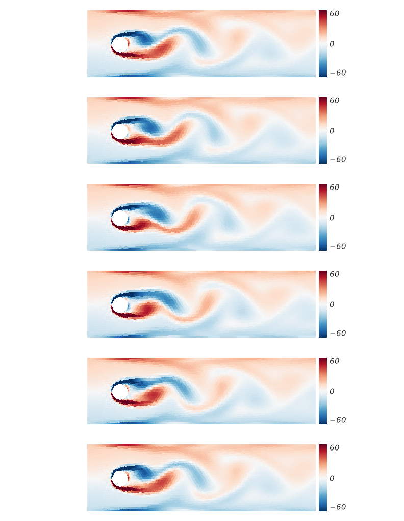
Vorticity w = dv/dx - du/dy, computed from the P1 element gradients — the exact derivative of the
velocity the run solved for, one value per cell. Near field only (x < 1.4); the colour range is set
from the wake, so the attached shear layer on the cylinder (which reaches |w| ~ 380) saturates.
Why the Strouhal number and not the drag
The 2D-1 tutorial reads drag and lift as the reaction conjugate to the cylinder's no-slip
constraint: fem.eval assembles the momentum residual with no essential elimination, and the sum over
the constrained DOFs is the force. That is the accurate route to a force from an FE solution — and it
is steady-only. The transient path publishes no free (pre-Dirichlet) residual, so fem.eval
refuses here.
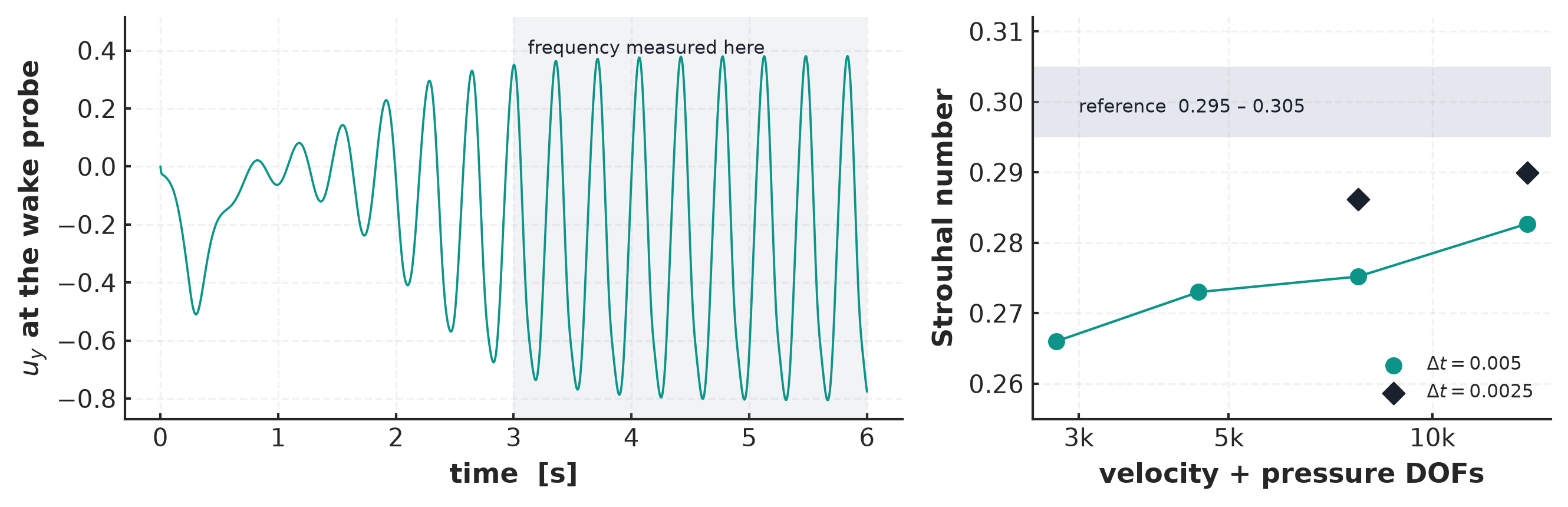
The Strouhal number needs no forces. It is the frequency of the transverse velocity at a fixed point in the wake, read straight out of the trajectory — so this benchmark is reachable anyway.
Measured
Equal-order P1/P1, BDF2, quasi-static tau. St converges monotonically from below under both
mesh and step refinement:
| mesh size | DOFs | dt |
scheme | St | vs 0.30 |
|---|---|---|---|---|---|
| 0.040 | 2,778 | 0.005 | BDF2 | 0.2660 | −11.3 % |
| 0.030 | 4,512 | 0.005 | BDF2 | 0.2730 | −9.0 % |
| 0.022 | 7,767 | 0.005 | BDF2 | 0.2752 | −8.3 % |
| 0.016 | 13,812 | 0.005 | BDF2 | 0.2827 | −5.8 % |
| 0.022 | 7,767 | 0.0025 | BDF2 | 0.2862 | −4.6 % |
| 0.016 | 13,812 | 0.0025 | BDF2 | 0.2899 | −3.4 % |
Halving dt at fixed mesh moves St about as much as refining the mesh at fixed dt, so neither
error dominates — this run is coarse in both, and the remaining 3.4 % is consistent with that rather
than with a defect in the formulation.
BDF2 versus backward Euler, on a real problem
Same mesh, same step, only the time scheme changed:
| scheme | St |
|---|---|
| backward Euler (θ = 1) | 0.2712 |
| BDF2 | 0.2752 |
Backward Euler is more damped, so it under-predicts the shedding frequency. This is the L-stable first-order scheme losing to the L-stable second-order one on exactly the quantity that a damped scheme distorts — the time-scheme note makes the same argument on a heat problem, and here it costs 1.5 % of a benchmark number.
A quasi-static residual, named as one
A fully consistent transient tau puts u_t in the momentum strong residual. That makes the
stabilisation a state-dependent mass c(u)·u_t. jno.solve.bdf2() marches such a mass (in its
non-conservative form, second order in time), but this tutorial keeps the quasi-static residual it was
built with — a real approximation, named as one. Whether the consistent form moves the Strouhal number
has not been measured.
Scope
- St is still 3.4 % low at the finest configuration run, and converging. This is not a converged benchmark result and is not presented as one.
- Drag and lift are not reported — see above. That is a jNO capability gap, not a choice.
- The wake probe sits at one point;
Stfrom zero crossings over the second half of the trajectory assumes the transient has died out by then, which the swing amplitude supports but does not prove. taucarries2/Δtand so assumes the fixed grid fromdomain(time=…). It is wrong underjno.solve.adaptive().linear=jno.solve.lu(backend="host")is not cosmetic: the device sparse factorisation ran out of cuSolver memory at 4,512 DOFs on an 8 GB card, and the host route was also 3.8× faster here.
Full script
"""**DFG benchmark 2D-2** -- unsteady vortex shedding past a cylinder at Re = 100, on stabilised
equal-order P1/P1 marched with BDF2, checked against the published Strouhal number.

    u_t + (u.grad)u - nu lap u + grad p = 0,   div u = 0,   Re = U_mean D / nu = 100

Configuration is Schäfer & Turek (1996), benchmark 2D-2 -- the same channel and cylinder as the
steady 2D-1 case, driven three times harder so the wake goes unstable and sheds a von Karman street:

    domain     [0, 2.2] x [0, 0.41] minus a disk of radius 0.05 at (0.2, 0.2)
    inflow     u = (4 U y (0.41 - y) / 0.41^2, 0),  U = 1.5  ->  U_mean = 1.0
    Strouhal   St = f D / U_mean,  reference ~ 0.30

This run exercises three things from the stabilised-flow work at once: the vector Laplacian in the
momentum strong residual, `dom.cell_metric` in `tau`, and `jno.solve.bdf2()` for the march.

**Why the Strouhal number and not the drag.** The 2D-1 tutorial reads forces as the reaction conjugate
to the cylinder's no-slip constraint -- `fem.eval` assembles the momentum residual with no essential
elimination and the sum over the constrained DOFs is the force. That readout is **steady-only**: the
transient path publishes no free (pre-Dirichlet) residual, so it is not available here. The Strouhal
number needs no forces at all -- it is the frequency of the transverse velocity at a fixed point in
the wake, which is read straight out of the trajectory.

**A quasi-static residual, named as one.** A fully consistent transient `tau` puts `u_t` in the strong
residual. That makes the stabilisation a *state-dependent mass* `c(u)*u_t`, which `jno.solve.bdf2()`
marches in its non-conservative form -- but the residual below stays quasi-static (no `u_t`), the form
this tutorial was built and measured with. That is a real approximation, named as one; whether the
consistent form moves the Strouhal number has not been measured.
"""

import os
import time

os.environ.setdefault("XLA_PYTHON_CLIENT_MEM_FRACTION", "0.6")

import jax

jax.config.update("jax_enable_x64", True)

import numpy as np  # noqa: E402

import jno  # noqa: E402

inner, grad, trace, lap = jno.np.inner, jno.np.grad, jno.np.trace, jno.np.laplacian

L, H = 2.2, 0.41
CX, CY, RR = 0.2, 0.2, 0.05
UMAX, NU = 1.5, 1e-3
UMEAN, DIA = 2.0 / 3.0 * UMAX, 2.0 * RR
EPS, C_I = 1e-9, 36.0
MS, T_END, NSTEPS = 0.022, 6.0, 1200  # ~90 s; the refinement table is in the tutorial page
ST_REF = 0.30  # Schäfer & Turek (1996), benchmark 2D-2

shape = jno.shape.rect(0, 0, L, H, size=MS) - jno.shape.disk(CX, CY, RR, size=MS / 5)
d = shape.domain(time=(0.0, T_END, NSTEPS + 1))
d.tag("inlet", lambda x, y: x < EPS)
d.tag("walls", lambda x, y: (y < EPS) | (y > H - EPS))
d.tag("cyl", lambda x, y: (x - CX) ** 2 + (y - CY) ** 2 < (RR + 1e-4) ** 2)

u, v = d.fem_symbols(value_shape=(2,), names=("u", "v"), order=1)  # equal order:
p, q = d.fem_symbols(names=("p", "q"), order=1)  # P1 velocity, P1 pressure
xi, yi, ti = d.variable("interior", split=True)
xin, yin, _ = d.variable("inlet", split=True)
xw, yw, _ = d.variable("walls", split=True)
xc, yc, _ = d.variable("cyl", split=True)
ci = d.variable("initial", split=True)

ub, vv = u.bind(x=xi, y=yi, t=ti), v.bind(x=xi, y=yi, t=ti)
gu, gv = grad(u, [xi, yi]), grad(v, [xi, yi])
gp, gq = grad(p, [xi, yi]), grad(q, [xi, yi])
pp, qq = p.bind(x=xi, y=yi, t=ti), q.bind(x=xi, y=yi, t=ti)

div = lambda gw: trace(gw)  # noqa: E731
adv = lambda gw, w: inner(gw, w, n_contract=1)  # noqa: E731

momentum = inner(ub.t, vv, 1) + inner(adv(gu, ub), vv, 1) + NU * inner(gu, gv, 2) - pp * div(gv)
continuity = -qq * div(gu)

dt = T_END / NSTEPS
G = d.cell_metric
gG = lambda a: inner(a, inner(G, a, n_contract=1), n_contract=1)  # noqa: E731
# The transient tau carries the step size. It assumes the FIXED grid from `domain(time=...)` and is
# wrong under `jno.solve.adaptive()`, where dt is chosen per step.
tau = jno.lag(((2.0 / dt) ** 2 + gG(ub) + C_I * NU**2 * inner(G, G, n_contract=2)) ** -0.5)
r_m = adv(gu, ub) - NU * lap(u, [xi, yi]) + gp  # quasi-static: no u_t (see the docstring)
momentum = momentum + tau * inner(adv(gv, ub), r_m, n_contract=1)  # SUPG -> momentum   (+)
continuity = continuity - tau * inner(gq, r_m, n_contract=1)  # PSPG -> continuity (-)

profile = 4.0 * UMAX * yin * (H - yin) / H**2
fem = jno.fem(
    [
        momentum,
        continuity,
        u(xin, yin)[0] - profile,
        u(xin, yin)[1] - 0.0,
        u(xw, yw)[0] - 0.0,
        u(xw, yw)[1] - 0.0,
        u(xc, yc)[0] - 0.0,
        u(xc, yc)[1] - 0.0,
        u(*ci)[0] - 0.0,
        u(*ci)[1] - 0.0,
    ]  # the outlet gets nothing: natural (do-nothing), which also sets the pressure level
)
assert fem.is_transient and not fem.is_linear
print(f"\nDFG 2D-2, vortex shedding at Re = {UMEAN * DIA / NU:.0f}: dofs={fem.dofs}, dt={dt:g}, T={T_END:g}")

t0 = time.time()
traj = np.asarray(
    fem.solve(
        nonlinear=jno.solve.newton(direct=True, rtol=1e-7, atol=1e-7),
        linear=jno.solve.lu(backend="host"),  # 3.8x faster here than the device factorisation
        time=jno.solve.bdf2(),  # second order AND L-stable
    ).fn()
)
print(f"  marched {traj.shape[0]} steps in {time.time() - t0:.0f} s ({1e3 * (time.time() - t0) / NSTEPS:.0f} ms/step)")

# ---- the Strouhal number, from the transverse velocity at a fixed wake probe --------------------
pts = np.asarray(fem.points)
probe = np.array([CX + 4 * RR, CY + RR])  # in the wake, off the centreline so the mode is visible
k = int(np.argmin(np.sum((pts - probe) ** 2, axis=1)))
ts = np.linspace(0.0, T_END, NSTEPS + 1)
uy = np.array([s[: fem.offsets[1]].reshape(len(pts), 2)[k, 1] for s in traj])

half = len(uy) // 2  # discard the start-up transient
tail, t_tail = uy[half:], ts[half:]
crossings = np.where(np.diff(np.sign(tail - tail.mean())))[0]
assert len(crossings) >= 4, f"the wake is not shedding ({len(crossings)} crossings) -- run longer"
period = 2.0 * np.mean(np.diff(t_tail[crossings]))
st = DIA / (UMEAN * period)

print(f"  probe at ({pts[k][0]:.3f}, {pts[k][1]:.3f}), u_y swing {tail.min():+.4f} .. {tail.max():+.4f}")
print(f"  shedding period {period:.4f} s  ->  f = {1 / period:.4f} Hz")
print(f"  St = {st:.4f}   reference ~ {ST_REF:.2f}   ({100 * (st - ST_REF) / ST_REF:+.1f}%)")

assert tail.max() - tail.min() > 0.1, "no sustained oscillation -- the wake did not go unstable"
assert 0.24 < st < 0.31, f"St = {st:.4f} is outside the band this discretisation converges through"
print("\nA von Karman street, at the right frequency to within the resolution of this run.")