Stokes 3D — Duct Past a Sphere
Creeping flow through a rectangular duct past a sphere, on inf-sup-stable Taylor–Hood tetrahedra — P2 velocity over P1 pressure:
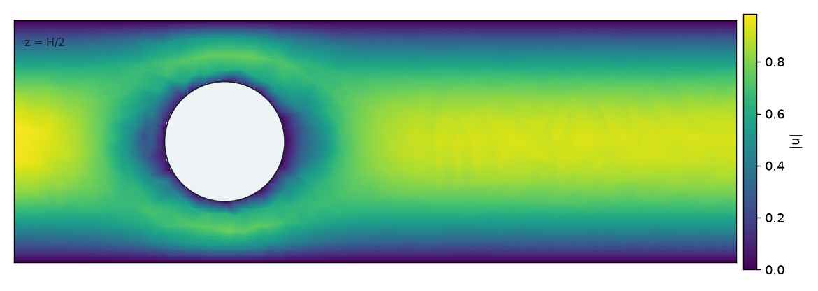
The geometry is CSG
The obstacle needs no bespoke mesh — subtract it:
duct = jno.shape.box(0, 0, 0, L, H, H) - jno.shape.sphere(CX, CY, CZ, R)
d = duct.size(0.06).domain()
The outflow is written by not writing it
The downstream face is left untagged. An untagged boundary is do-nothing in jNO, which is exactly the traction-free condition Stokes flow wants at an outlet:
d.tag("inlet",  lambda x, y, z: x < EPS)
d.tag("walls",  lambda x, y, z: (y < EPS) | (y > H - EPS) | (z < EPS) | (z > H - EPS))
d.tag("sphere", lambda x, y, z: (x - CX)**2 + (y - CY)**2 + (z - CZ)**2 < (R + 1e-3)**2)
That also settles the pressure level, which is why this problem carries no p.pin(). An
enclosed flow — every wall Dirichlet — has a constant pressure null space and does need a gauge;
use p.pin(mean=True) there, not a point pin, or the pressure will not converge in 3-D.
Drag as a reaction, not a surface integral
fem.eval(term, u) assembles the momentum residual with no essential elimination applied, so
the sum over the sphere's constrained DOFs is the force holding it in place. The force the fluid
exerts is its negative:
R_free     = np.asarray(fem.eval(momentum, sol))
reaction_x = float(R_free[fem.region_dofs("sphere", field=u, component=0)].sum())
drag       = -reaction_x
This is the accurate way to get a force out of a finite element solution — more so than integrating the stress over the surface, because the reaction is exactly conjugate to the constraint.
What to notice
- It is a saddle system.
fem.solve()warns if you point the matrix-free default at it; a direct factorization is used here, and past this size the block/Schur preconditioners injno.precondare what scale. - The peak speed does not rise. A centred sphere blocks the fast core of a parabolic profile and pushes fluid into the slower corners, so the maximum speed in the sphere's plane (0.94) is below the inflow peak (1.00). Blockage does not always mean acceleration.
- The drag is a confined-sphere drag. At 3.36× the unbounded Stokes-law value \(6\pi\mu R U\), it reflects a duct only twice the sphere diameter across. That ratio is a sanity band, not a benchmark match — the wall correction at 50 % blockage is large.
Full script
"""**3-D Stokes flow** through a rectangular duct past a sphere -- creeping flow in three dimensions
on inf-sup-stable Taylor-Hood tetrahedra (P2 velocity, P1 pressure).

    -nu lap u + grad p = 0,   div u = 0

Three things worth noticing, all of them 3-D-specific:

* the **geometry is CSG** -- a box minus a sphere -- so the obstacle needs no bespoke mesh;
* the **outflow is natural**. Nothing is written for the downstream face: an untagged boundary is
  do-nothing in jNO, which is exactly the traction-free condition Stokes flow wants there. It also
  fixes the pressure LEVEL, which is why this problem needs no `p.pin()` at all -- an enclosed flow
  (every wall Dirichlet) does, and should use `p.pin(mean=True)`;
* the **drag on the sphere is read as a reaction**, not by integrating stress over its surface.
  `fem.eval(term, u)` assembles the momentum residual with no essential elimination applied, and the
  sum over the sphere's constrained DOFs is the force the fluid exerts on it -- the accurate way to
  get a force out of a finite element solution.
"""

import os

os.environ.setdefault("XLA_PYTHON_CLIENT_MEM_FRACTION", "0.6")  # play nice on a shared GPU

import jax

jax.config.update("jax_enable_x64", True)  # the assembler builds in float64

import numpy as np  # noqa: E402

import jno  # noqa: E402

inner, grad, trace = jno.np.inner, jno.np.grad, jno.np.trace

NU = 1.0  # creeping flow: the Stokes limit, no convective term at all
L, H = 1.2, 0.4  # duct length and (square) cross-section
CX, CY, CZ, R = 0.35, 0.2, 0.2, 0.1  # sphere centre and radius
U0 = 1.0  # peak inflow speed
EPS = 1e-9

duct = jno.shape.box(0, 0, 0, L, H, H) - jno.shape.sphere(CX, CY, CZ, R)
d = duct.size(0.06).domain()

# Boundary regions. The downstream face is deliberately left untagged -> natural (do-nothing).
d.tag("inlet", lambda x, y, z: x < EPS)
d.tag("walls", lambda x, y, z: (y < EPS) | (y > H - EPS) | (z < EPS) | (z > H - EPS))
d.tag("sphere", lambda x, y, z: (x - CX) ** 2 + (y - CY) ** 2 + (z - CZ) ** 2 < (R + 1e-3) ** 2)

u, v = d.fem_symbols(value_shape=(3,), names=("u", "v"), order=2)  # P2 velocity
p, q = d.fem_symbols(names=("p", "q"), order=1)  # P1 pressure
xi, yi, zi = d.variable("interior", split=True)[:3]
xin, yin, zin = d.variable("inlet", split=True)[:3]
xw, yw, zw = d.variable("walls", split=True)[:3]
xs, ys, zs = d.variable("sphere", split=True)[:3]

gu, gv = grad(u, [xi, yi, zi]), grad(v, [xi, yi, zi])
pp, qq = p.bind(x=xi, y=yi, z=zi), q.bind(x=xi, y=yi, z=zi)
momentum = NU * inner(gu, gv, n_contract=2) - pp * trace(gv)
inflow = U0 * 16.0 * yin * (H - yin) * zin * (H - zin) / H**4  # parabolic in both cross-stream axes

fem = jno.fem(
    [
        momentum,
        -qq * trace(gu),
        u(xin, yin, zin)[0] - inflow,  # driven face
        u(xin, yin, zin)[1] - 0.0,
        u(xin, yin, zin)[2] - 0.0,
        *[u(xw, yw, zw)[k] - 0.0 for k in range(3)],  # no-slip duct walls
        *[u(xs, ys, zs)[k] - 0.0 for k in range(3)],  # no-slip sphere
    ]
)
off = fem.offsets
print(f"\n3-D Stokes duct past a sphere: dofs={fem.dofs} (velocity {off[1]}, pressure {fem.dofs - off[1]})")

# A saddle system: use a direct factorization rather than the matrix-free default (fem.solve() says
# so itself if you forget). Past this size the block/Schur route in jno.precond is what scales.
sol = np.asarray(fem.solve(linear=jno.solve.lu(backend="host")))
vel = sol[off[0] : off[1]].reshape(-1, 3)
pre = sol[off[1] :]
pts = np.asarray(fem.field_points[0])

# ---- drag on the sphere, as the reaction conjugate to its no-slip constraint ----
# `fem.eval` returns the INTERNAL force at every DOF. At a constrained DOF that is the reaction --
# the force holding the sphere in place -- so the force the fluid exerts on the sphere is its
# negative. The pressure field confirms the sign independently: it is far higher upstream of the
# sphere than downstream, which pushes the sphere downstream (+x).
R_free = np.asarray(fem.eval(momentum, sol))  # residual with NO essential elimination applied
reaction_x = float(R_free[fem.region_dofs("sphere", field=u, component=0)].sum())
drag = -reaction_x

ppts = np.asarray(fem.field_points[1])
up = (ppts[:, 0] > CX - R - 0.06) & (ppts[:, 0] < CX - R)
dn = (ppts[:, 0] > CX + R) & (ppts[:, 0] < CX + R + 0.06)
speed = np.linalg.norm(vel, axis=1)
stokes_law = 6.0 * np.pi * NU * R * U0  # the UNBOUNDED sphere, for scale only -- see below

print(f"  peak speed {speed.max():.4f}   pressure drop across the duct {pre.max() - pre.min():.2f}")
print(f"  drag on the sphere Fx = {drag:+.4f}   ({drag / stokes_law:.2f}x the unbounded Stokes-law value)")
print(f"  mean pressure upstream {pre[up].mean():+.1f} vs downstream {pre[dn].mean():+.1f}")

assert drag > 0.0, f"the sphere must resist the flow, got Fx = {drag:.3e}"
assert pre[up].mean() > pre[dn].mean(), "pressure must fall across the obstacle"
# The duct is only twice the sphere diameter across, so this is a STRONGLY confined sphere and the
# drag is several times the unbounded Stokes-law value 6*pi*mu*R*U. That is a sanity band, not a
# benchmark: the wall correction at 50% blockage is large and this is not a match to any published
# number. (The peak speed does NOT rise above the inflow peak, incidentally -- a centred sphere
# blocks the fast core of a parabolic profile and pushes fluid into the slower corners.)
assert 2.0 < drag / stokes_law < 6.0, f"drag {drag:.3f} is not a plausible confined-sphere value"