Phase-Field Fracture, SENT — the whole study as a term list

Download .py All tutorials

A single-edge-notched specimen pulled in tension, with the crack regularized into a damage field \(d\in[0,1]\). What makes this worth its own tutorial is not the physics — that is the standard second-order AT2 model — but that none of it is driven from outside jno.fem. The coupled system, the irreversible history, the bound on the damage, the alternating solver and the non-uniform load path are all either a term in the list or a slot on fem.solve.

what	how
the stress is the energy derivative	`sigma = jno.np.diff(psi, eps(u))`
irreversible history \(H=\max_\tau \psi^+\)	`Hs.evolves(maximum(Hs.i(-1), psi_p))` — on a coupled system
damage is a fraction	`dm.bounds(0.0, 1.0)` — an inequality, in the term list
the energy is non-convex in \((u,d)\) jointly	`nonlinear=jno.solve.staggered([u, dm])`
the load path is not uniform	`tau=jno.solve.adaptive(limit=[(dm, 0.5)])`
the reaction force	`fem.eval(momentum, u_k)[grip]`

The model

The elastic energy is split volumetric/deviatoric so only the tensile part drives damage and a closed crack still carries compression (Amor, Marigo & Maurini, JMPS 57 (2009) 1209–1229):

\[ \psi^+ = \tfrac12 K \langle \operatorname{tr}\varepsilon\rangle_+^2 + \mu\, \varepsilon_{\text{dev}}\!:\!\varepsilon_{\text{dev}}, \qquad \sigma = \frac{\partial}{\partial\varepsilon}\Big[ g(d)\,\psi^+ + \psi^- \Big]. \]

That last line is written literally — jno.np.diff differentiates the energy, so there is no hand-derived stress anywhere. Irreversibility comes from the history field \(H=\max_\tau\psi^+\), so a crack cannot heal (Miehe, Welschinger & Hofacker, IJNME 83 (2010) 1273–1311), and the damage equation is the standard AT2 form \((G_c/\ell)\,d - G_c\ell\,\Delta d = 2(1-d)H\).

The notch is cut, not painted on: a real slit removed from the geometry with jno.shape, so the stress concentration at its tip is the mesh's own and the damage field needs no seeding.

plate = jno.shape.rect(0.0, 0.0, 1.0, 1.0, size=h)
slit  = jno.shape.rect(-0.01, 0.5 - w_slit, 0.5, 0.5 + w_slit, size=h)
dom   = (plate - slit).domain(tau=(0.0, 1.0, NOUT))     # tau: the pseudo-time LOAD path

Loading is displacement-controlled — u(*ct)[1] - DELTA * ct[-1], the grip displacement ramped in \(\tau\). That is not a stylistic choice: under load control a brittle specimen snaps at the peak and there is no branch left to follow, so a softening response can only be traced by prescribing the grip.

What it shows, and what it refuses to

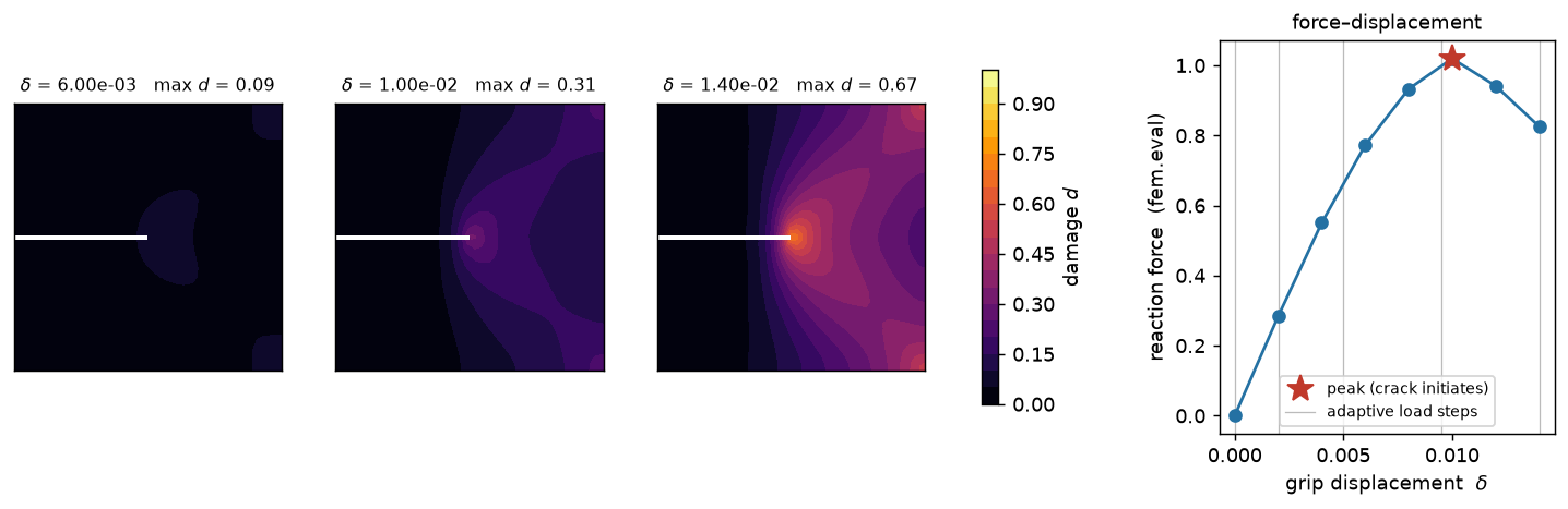
Damage initiates at the notch tip and grows smoothly while the load rises. That part is stable, and the adaptive controller resolves it — the schedule comes back as [0, 0.143, 0.357, 0.679, 1.0], taking large steps while nothing happens and cutting as the tip loads up. The reaction rises to a peak and then softens, read straight off fem.eval.

Propagation across the ligament is not stable for this geometry. Ask for a finer resolution of the same path and the controller cannot deliver one:

tighter limit (0.25): refused, and named the unstable branch rather than returning a path

That is the correct answer, not a solver failure. Past the peak there is no nearby equilibrium, so no amount of load-step refinement finds one — verified separately: a 5× finer uniform grid gives the same jump, the crack tip going from \(x=0.05\) to \(x=1.0\) in a single increment either way. Following an unstable branch needs arc-length (dissipation-controlled) continuation, which jNO does not have. The alternative to reporting this is grinding to the step floor and returning a plausible-looking path that never happened.

Damage field at three load levels, initiating ahead of the notch tip and localizing into a band on the crack plane, beside the force–displacement curve with its peak marked and the adaptive load steps shown as vertical rules.

Notes on the numbers

The bound is solved, not clipped — damage stays in \([0,1]\) through the KKT conditions of the variational inequality, and is monotone because the history field is a running max.
fem.block_index(dm) resolves the damage block: field order is first appearance in the term walk, and the degradation factor puts dm ahead of u. Never hardcode the index.
The degradation floor \(\eta\) is still needed even with the bound: at \(d=1\) exactly, \((1-d)^2\) makes the displacement block singular. The bound keeps \(d\) in range; it does not make the operator well-posed.
AT2 has no elastic threshold, so \(d>0\) everywhere from the first increment. Statements about localization have to be about substantial damage, not about where the field is nonzero.
The two stragglers outside the crack band are the grip corners, where a fully clamped edge meets a free lateral edge and the elastic field is singular — a property of the boundary conditions rather than of the model.

For the fourth-order regularization on a biharmonic (Morley/Argyris) element, see Brittle Fracture — 4th-order phase-field; that model needs a \(C^1\)-ish space, which the load-path march does not yet carry.

Full script

"""Brittle fracture, second-order phase-field — a single-edge-notched tension test, as a term list.

The whole study is `jno.fem([...])` plus `fem.solve(...)`: a coupled displacement/damage system, an
irreversible per-quadrature-point history, a bound, an alternating solver and an adaptive load path.
Nothing is hand-rolled around the FEM.

Six pieces carry it, and each one is a formula or a slot rather than a driver:

| what | how |
|---|---|
| the stress **is** the energy derivative | `sig = jno.np.diff(psi, eps(u))` |
| irreversible history `H = max_tau psi+` | `Hs.evolves(maximum(Hs.i(-1), psi_p))` — a coupled state |
| damage is a fraction | `dm.bounds(0.0, 1.0)` — an inequality, in the term list |
| the energy is non-convex in `(u, d)` jointly | `nonlinear=jno.solve.staggered([u, dm])` |
| the load path is not uniform | `tau=jno.solve.adaptive(limit=...)` |
| the reaction force | `fem.eval(momentum, u_k)` on the loaded edge |

**Model.** A cracking solid minimizes elastic + fracture energy; the sharp crack is regularized into a
damage field `d in [0,1]` over a length `ell` (Bourdin, Francfort & Marigo, *J. Elasticity* **91**
(2008) 5-148). The elastic energy is split volumetric/deviatoric so only the *tensile* part drives
damage and a closed crack still carries compression (Amor, Marigo & Maurini, *JMPS* **57** (2009)
1209-1229). Irreversibility comes from the history field `H = max_tau psi+`, so a crack cannot heal
(Miehe, Welschinger & Hofacker, *IJNME* **83** (2010) 1273-1311). The regularization is the standard
second-order AT2, whose damage equation is `(Gc/ell) d - Gc*ell*lap(d) = 2(1-d)H`.

**What this run shows, and what it refuses to.** Damage initiates at the notch tip and grows smoothly
while the load rises — that part is stable, and the adaptive controller resolves it, taking large steps
while nothing happens and small ones as the tip loads up. Propagation across the ligament is *not*
stable for this geometry: once the crack runs there is no nearby equilibrium, and the second solve below
shows the controller diagnosing exactly that instead of returning a plausible-looking wrong path.
Following an unstable branch needs arc-length control, which jNO does not have — see the closing note.
"""

import os

import jax

jax.config.update("jax_enable_x64", True)

import numpy as np

import jno

n = jno.np
inner, sym, grad, trace, maximum, minimum, diff, ident = (
    n.inner,
    n.sym,
    n.grad,
    n.trace,
    n.maximum,
    n.minimum,
    n.diff,
    n.identity,
)

# --- material, regularization, mesh -----------------------------------------------------------------
E, nu = 210.0, 0.3  # stiff, brittle
lam, mu = E * nu / ((1 + nu) * (1 - 2 * nu)), E / (2 * (1 + nu))
Kpl = lam + mu  # plane-strain bulk modulus (the volumetric part of the split)
Gc, ell, eta = 2.7e-3, 0.06, 1e-6  # toughness, regularization length, degradation floor
h, w_slit = 0.03, 0.010  # mesh size; slit half-width (h/ell < 1/2 resolves the damage band)
DELTA, NOUT = 1.4e-2, 8  # peak grip displacement, reported load levels

# The notch is CUT, not painted on: a real slit in the geometry, so the stress concentration at its tip
# is the mesh's own and no seeding of the damage field is needed.
plate = jno.shape.rect(0.0, 0.0, 1.0, 1.0, size=h)
slit = jno.shape.rect(-0.01, 0.5 - w_slit, 0.5, 0.5 + w_slit, size=h)
dom = (plate - slit).domain(tau=(0.0, 1.0, NOUT))  # tau: the pseudo-time LOAD path
dom.tag("bot", lambda x, y: y < 1e-9)
dom.tag("top", lambda x, y: y > 1 - 1e-9)
co, cb, ct = (dom.variable(r, split=True) for r in ("interior", "bot", "top"))
X = [co[0], co[1]]

u, phi = dom.fem_symbols(value_shape=(2,))  # displacement (vector)
dm, q = dom.fem_symbols()  # damage (scalar)
Hs, _ = dom.fem_symbols(value_shape=())  # the history state — never solved for, only evolved

# --- the energy, written once; the stress follows by differentiating it ------------------------------
I2 = ident(2)
eps = lambda v: sym(grad(v, X))  # noqa: E731
e_u = eps(u)
tr_u = trace(e_u)
dev_u = e_u - tr_u / 2 * I2
psi_p = 0.5 * Kpl * maximum(tr_u, 0.0) ** 2 + mu * inner(dev_u, dev_u, 2)  # tensile: drives damage
psi_m = 0.5 * Kpl * minimum(tr_u, 0.0) ** 2  # compressive: never degraded
g_d = (1.0 - dm) ** 2 + eta  # AT2 degradation, floored so the u block stays non-singular
sigma = diff(g_d * psi_p + psi_m, e_u)  # <-- no hand-derived stress anywhere

momentum = inner(sigma, eps(phi), 2)
damage = (Gc / ell) * dm * q + Gc * ell * inner(grad(dm, X), grad(q, X), 1) - 2.0 * (1.0 - dm) * Hs.i(-1) * q

fem = jno.fem(
    [
        momentum,  # equilibrium                     (test phi)
        damage,  # AT2 damage evolution            (test q)
        Hs.evolves(maximum(Hs.i(-1), psi_p)),  # irreversibility  (a named update)
        dm.bounds(0.0, 1.0),  # damage is a fraction            (an inequality)
        u(*cb)[0] - 0.0,
        u(*cb)[1] - 0.0,  # bottom grip clamped
        u(*ct)[0] - 0.0,
        u(*ct)[1] - DELTA * ct[-1],  # top grip pulled: DISPLACEMENT control, ramped in tau
    ]
)

alt = jno.solve.staggered([u, dm], max_sweeps=60, rtol=1e-7, atol=1e-9)
traj = np.asarray(fem.solve(nonlinear=alt, tau=jno.solve.adaptive(limit=[(dm, 0.5)], max_steps=120)))
schedule = fem.tau_schedule

# --- readouts ----------------------------------------------------------------------------------------
i_u, i_d = fem.block_index(u), fem.block_index(dm)  # block order is first appearance, so ASK
dmg = traj[:, fem.blocks[i_d]]
pts_d = np.asarray(fem.field_points[i_d])
grip = fem.region_dofs("top", field=u, component=1)  # the loaded edge's y DOFs

# The reaction is the momentum residual at the solution, restricted to the grip — `fem.eval` assembles
# it un-eliminated, which every solve path would otherwise have zeroed on exactly those rows.
reaction = np.array([float(np.asarray(fem.eval(momentum, traj[k]))[grip].sum()) for k in range(traj.shape[0])])
delta = DELTA * np.linspace(0.0, 1.0, NOUT)
tip = np.array([pts_d[dmg[k] > 0.5, 0].max() if (dmg[k] > 0.5).any() else 0.5 for k in range(traj.shape[0])])
k_peak = int(np.argmax(np.abs(reaction)))

print("\nPhase-field SENT, second-order AT2 (P1 Lagrange, coupled u/d + per-QP history):")
print(f"  mesh: {np.asarray(dom.mesh.points).shape[0]} nodes, {fem.dofs} dofs   h/ell = {h / ell:.2f}")
print(f"  adaptive load path: {len(schedule)} steps at tau = {np.round(schedule, 3)}")
print(f"  damage range over the path: [{dmg.min():.3e}, {dmg.max():.3f}]   (bounds, not clipping)")
print(f"  peak reaction {abs(reaction[k_peak]):.4e} at delta = {delta[k_peak]:.4e}; final {abs(reaction[-1]):.4e}")
print(f"  damage max per step: {np.round(dmg.max(axis=1), 3)}")

# --- asserts: the bound holds exactly; damage initiates at the tip, in-band; the specimen softens ------
assert dmg.min() > -1e-12 and dmg.max() < 1.0 + 1e-12, f"damage left [0,1]: [{dmg.min():.2e}, {dmg.max():.3f}]"
assert dmg.max() > 0.5, "no damage developed — nothing to report"
assert np.all(np.diff(dmg.max(axis=1)) > -1e-9), "damage must be monotone — the history field is irreversible"
hot = dmg[-1] > 0.5
apex = pts_d[int(np.argmax(dmg[-1]))]
assert abs(apex[1] - 0.5) < ell and apex[0] > 0.5, f"damage must peak ahead of the notch tip, got {apex.round(3)}"
# Most of the damage lies in the band; the stragglers are the two GRIP CORNERS, where a fully clamped
# edge meets a free lateral edge and the elastic field is singular. That is a property of the boundary
# conditions, not of the model — a real rig loads through a compliant grip, and a phase-field study
# either rounds those corners or excludes them from the damage region.
inband = np.abs(pts_d[hot, 1] - 0.5) < 4 * ell
assert inband.mean() > 0.8, f"damage must localize into a band on the crack plane ({100 * inband.mean():.0f}% in band)"
assert tip[-1] > 0.5 + ell, f"the crack must advance past the notch tip: {tip[-1]:.3f}"
assert len(schedule) >= 4 and np.ptp(np.diff(schedule)) > 1e-3, "the load path must actually adapt"
assert abs(reaction[-1]) < 0.9 * abs(reaction[k_peak]), "the specimen must soften after the peak"

# --- the instability, diagnosed rather than mis-resolved ---------------------------------------------
# Ask for a *finer* resolution of the same path and the controller cannot deliver it — not because the
# step is too big, but because past the peak there is no nearby equilibrium at all. Refining the load
# step cannot find one (verified separately: a 5x finer uniform grid gives the same jump), and the
# error says so instead of grinding to the floor and returning a plausible path.
try:
    fem.solve(nonlinear=alt, tau=jno.solve.adaptive(limit=[(dm, 0.25)], max_steps=120))
    verdict = "converged — this geometry's propagation was stable after all"
except RuntimeError as exc:
    assert "UNSTABLE" in str(exc) and "arc-length" in str(exc), str(exc)
    verdict = "refused, and named the unstable branch rather than returning a path"
print(f"  tighter limit (0.25): {verdict}")