2D Helmholtz with a PML (complex FEM)

Download .py Back to chapter

A time-harmonic scattering / radiation problem: a point source radiates outward and a Perfectly Matched Layer (PML) absorbs the outgoing wave with no reflection, so a truncated box behaves like open space. The PML is a complex coordinate stretch \(s = 1 + i\,\sigma(x)/k\) (\(\sigma\) ramps up in a frame, \(0\) in the physical core) — so the weak form has complex coefficients and the solution \(u\) is complex.

Complex weak form via 1j

A 1j coefficient (Python's native imaginary unit) makes the weak form complex. jno.fem then solves the problem with a real-equivalent method (it splits each term into real \(\mathrm{Re}\)/\(\mathrm{Im}\) sub-forms, assembles both through the ordinary real FEM path, solves the block \(\begin{bmatrix}A_r&-A_i\\A_i&A_r\end{bmatrix}\begin{bmatrix}u_r\\u_i\end{bmatrix}=\begin{bmatrix}b_r\\b_i\end{bmatrix}\) and recombines to \(u=u_r+i\,u_i\)). The PML's anisotropic stretched operator reads directly:

Sx, Sy = 1.0 + 1j * sx / k, 1.0 + 1j * sy / k  # complex coordinate stretch
weak = (Sy / Sx) * (ui.x * vi.x) + (Sx / Sy) * (ui.y * vi.y) - k**2 * Sx * Sy * (u * vi) - src * vi
fem = jno.fem([weak, u(xb, yb) - 0.0], quad_degree=3)  # detects complex -> real-equivalent solve
u = fem.solve()                                        # complex128 field u_r + i u_i

The result

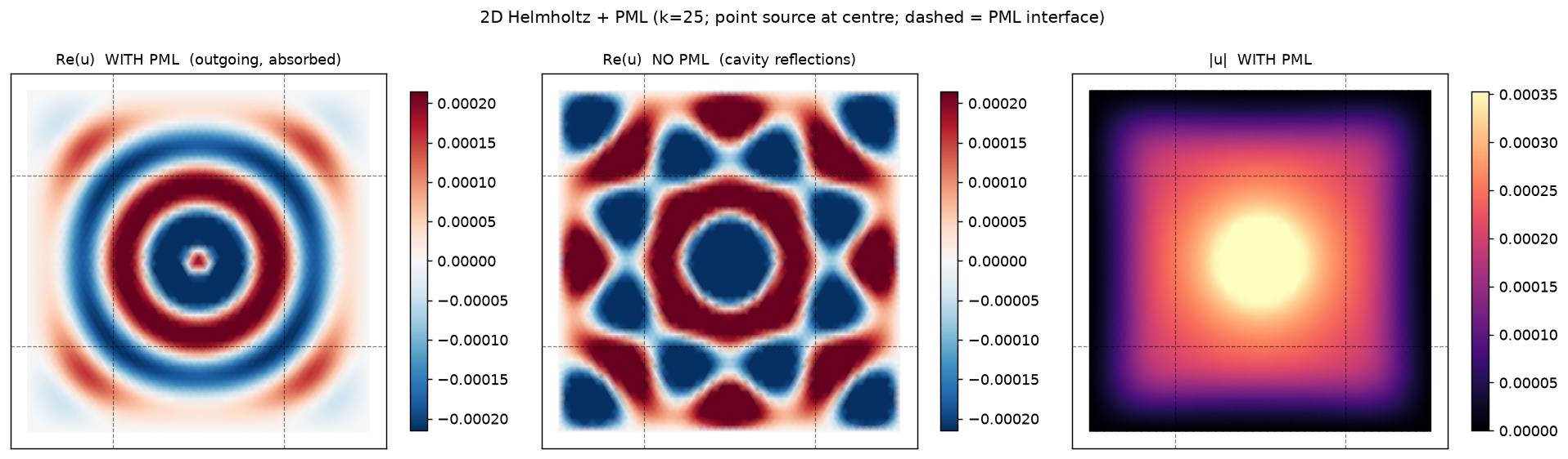
Left: \(\mathrm{Re}(u)\) with the PML — concentric outgoing wavefronts, smoothly absorbed at the dashed PML interface. Middle: the same problem without the PML (\(\sigma=0\), \(u=0\) walls) — the wave reflects and resonates. Right: \(|u|\), decaying into the absorbing frame.

What to notice

• A complex coefficient (a 1j) is the only signal needed — fem.is_complex is True and fem.solve() returns a complex128 field.
• The complex solve uses the real-equivalent block; the underlying real FEM backend is never asked to assemble a complex matrix.
• PML quality, no analytic solution required: a converged PML's physical-core field is independent of the absorber strength \(\sigma_0\) — here the relative change from \(\sigma_0=40\) to \(60\) is \(\sim 9\times10^{-4}\), i.e. the truncation is effectively reflection-free.

Full script

"""09 - 2D Helmholtz with a Perfectly Matched Layer (PML), via jno's complex FEM.

A point source radiates outward; a PML frame absorbs the outgoing wave with no reflection, so the
truncated box behaves like open space. The PML is a *complex coordinate stretch* s = 1 + i sigma/k
(sigma ramps up in the frame, 0 in the physical core) -- so the weak form has complex coefficients.

jno.fem detects the complex form (a ``1j`` coefficient) and solves it via the
real-equivalent block (it splits each term into real Re/Im sub-forms, assembles both through the
ordinary REAL assembly path, solves [[A_r,-A_i],[A_i,A_r]], and recombines to u = u_r + i u_i). The
assembler is never asked to build a complex matrix.

PML-quality check (no analytic solution needed): a *converged* PML's physical-core field does not
depend on the absorber strength sigma0 -- a poor / absent PML reflects and changes with sigma0.
The script also renders the field (the actual computed solution): the outgoing wave absorbed by
the PML, versus the reflecting cavity without it.
"""

import os

os.environ["MPLBACKEND"] = "Agg"

import jax

jax.config.update("jax_enable_x64", True)  # the real-equivalent block is float64

from pathlib import Path  # noqa: E402

import matplotlib.pyplot as plt  # noqa: E402
import matplotlib.tri as mtri  # noqa: E402
import numpy as np  # noqa: E402
from shapely.geometry import box  # noqa: E402

import jno  # noqa: E402

L, w, k = 1.0, 0.25, 25.0  # box, PML frame width, wavenumber (~4 wavelengths across the core)
relu = lambda z: jno.np.maximum(z, 0.0)  # noqa: E731


def solve_pml(sigma0):
    """Complex PML Helmholtz at absorber strength sigma0 (sigma0 = 0 -> no PML, u=0 cavity)."""
    d = jno.domain(box(0.0, 0.0, L, L), mesh_size=0.022)
    u, phi = d.fem_symbols()
    xi, yi, _ = d.variable("interior", split=True)
    xb, yb, _ = d.variable("boundary", split=True)
    ui, vi = u.bind(x=xi, y=yi), phi.bind(x=xi, y=yi)
    sx = sigma0 * (relu(w - xi) ** 2 + relu(xi - (L - w)) ** 2) / w**2  # quadratic PML profile, per axis
    sy = sigma0 * (relu(w - yi) ** 2 + relu(yi - (L - w)) ** 2) / w**2
    Sx, Sy = 1.0 + 1j * sx / k, 1.0 + 1j * sy / k  # complex coordinate stretch
    src = jno.np.exp(-(((xi - 0.5) ** 2 + (yi - 0.5) ** 2) / (2 * 0.025**2)))  # ~point source at centre
    weak = (Sy / Sx) * (ui.x * vi.x) + (Sx / Sy) * (ui.y * vi.y) - k**2 * Sx * Sy * (u * vi) - src * vi
    fem = jno.fem([weak, u(xb, yb) - 0.0], quad_degree=3)  # u = 0 outer wall (PML absorbs first)
    return fem, np.asarray(fem.solve())


fem, u_pml = solve_pml(40.0)
_, u_strong = solve_pml(60.0)  # 1.5x absorber -> physical core must be unchanged
_, u_off = solve_pml(0.0)  # no PML: the wave reflects off the walls
pts = np.asarray(fem.points)
tris = np.asarray(fem.domain.built_mesh.cells_dict["triangle"])

core = (pts[:, 0] > w) & (pts[:, 0] < L - w) & (pts[:, 1] > w) & (pts[:, 1] < L - w)
sigma_insens = float(np.linalg.norm(u_pml[core] - u_strong[core]) / np.linalg.norm(u_pml[core]))
print("\n2D Helmholtz + PML via complex jno.fem")
print(f"  complex solve: dofs={fem.dofs}  dtype={u_pml.dtype}")
print(f"  PML reflection-free (sigma-insensitivity rel-L2, 40 vs 60): {sigma_insens:.3e}")

# ---- render the actual computed field (no invented structure) ----
triang = mtri.Triangulation(pts[:, 0], pts[:, 1], tris)
wave = float(np.percentile(np.abs(np.real(u_pml)), 88))  # clip so the wavefronts show past the source peak
fig, ax = plt.subplots(1, 3, figsize=(15, 4.6))
panels = [
    ("Re(u)  WITH PML  (outgoing, absorbed)", np.real(u_pml), "RdBu_r", (-wave, wave)),
    ("Re(u)  NO PML  (cavity reflections)", np.real(u_off), "RdBu_r", (-wave, wave)),
    ("|u|  WITH PML", np.abs(u_pml), "magma", (0.0, float(np.percentile(np.abs(u_pml), 95)))),
]
for a, (title, field, cmap, (vmn, vmx)) in zip(ax, panels):
    tpc = a.tripcolor(triang, field, cmap=cmap, shading="gouraud", vmin=vmn, vmax=vmx)
    fig.colorbar(tpc, ax=a, shrink=0.8)
    for off in (w, L - w):
        a.axvline(off, ls="--", c="k", lw=0.7, alpha=0.5)
        a.axhline(off, ls="--", c="k", lw=0.7, alpha=0.5)
    a.set_title(title, fontsize=10)
    a.set_aspect("equal")
    a.set_xticks([])
    a.set_yticks([])
fig.suptitle(f"2D Helmholtz + PML (k={k:g}; point source at centre; dashed = PML interface)", fontsize=11)
fig.tight_layout()
fig.savefig(Path(__file__).parents[2] / "assets" / "helmholtz_pml_2d.png", dpi=130, bbox_inches="tight")  # docs/assets

assert fem.is_complex and np.iscomplexobj(u_pml) and not bool(np.isnan(u_pml).any())
assert sigma_insens < 1e-2, f"PML not reflection-free: {sigma_insens:.3e}"