Time-harmonic 2D Maxwell — in-plane vector \(E\) (complex vector FEM)

Download .py Back to chapter

Frequency-domain Maxwell for the in-plane electric field \(E = (E_x, E_y)\) (TE polarisation) is the curl–curl equation

\[ \nabla\times(\nabla\times E) \;-\; k^2\,E \;=\; J, \qquad k^2 = \omega^2\mu\varepsilon, \]

with \(E\) complex-valued (\(k^2\) is complex in a lossy medium). This is the genuine vector complex problem — not a scalar Helmholtz.

A complex field is one symbol — complex=True

domain.fem_symbols(..., complex=True) returns a complex trial/test. You write the weak form once with ordinary complex algebra (* is the complex product, 1j is just the imaginary unit, .real / .imag / .conj / .dot), and jno.fem lowers weak.real for you. Under the hood a complex vector is carried as two coupled real vector fields \((E_r, E_i)\) — \(4\) real DOFs per node — and the real-part lowering lands on the coupled multifield system jno.fem already assembles for the two-temperature and Stokes examples. There is no separate "complex solver": one notion of complex, 1j everywhere, the tracer carries the rest.

E, v = d.fem_symbols(value_shape=(2,), complex=True, order=2)   # a complex vector field + its test
Eb, vb = E.bind(x=x, y=y), v.bind(x=x, y=y)

curl = lambda F: F.x[1] - F.y[0]        # 2-D scalar curl  ∂Fy/∂x − ∂Fx/∂y
div  = lambda F: F.x[0] + F.y[1]
k2 = KR + 1j*KI                         # complex coefficient — a plain Python complex
J  = jno.complex(Jr, Ji)                # complex forcing (data) = re + 1j*im

weak = curl(Eb)*curl(vb) + s*div(Eb)*div(vb) - k2*Eb.dot(vb) - J.dot(vb)   # `*` is the complex product
fem  = jno.fem([weak.real, *boundary_conditions])   # `.real` lowers onto the coupled real solve

weak.real is one expression whose real part mixes both test fields; jno.fem distributes it into the per-field (\(E_r\), \(E_i\)) blocks automatically. Two details for a nodal (Lagrange) discretisation of curl–curl:

• the scalar curl is F.x[1] - F.y[0] — grad-then-index, because the backend differentiates the trial, not a component of it (F[1].x is not supported);
• nodal elements need a grad–div penalty \(+\,s\,(\nabla\!\cdot E)(\nabla\!\cdot v)\) to suppress the spurious curl kernel. It is consistent here because the exact field is divergence-free, so the penalty vanishes at the solution. With it, P1 converges \(\sim\!\mathcal{O}(h^2)\) and P2 is essentially exact.

The result

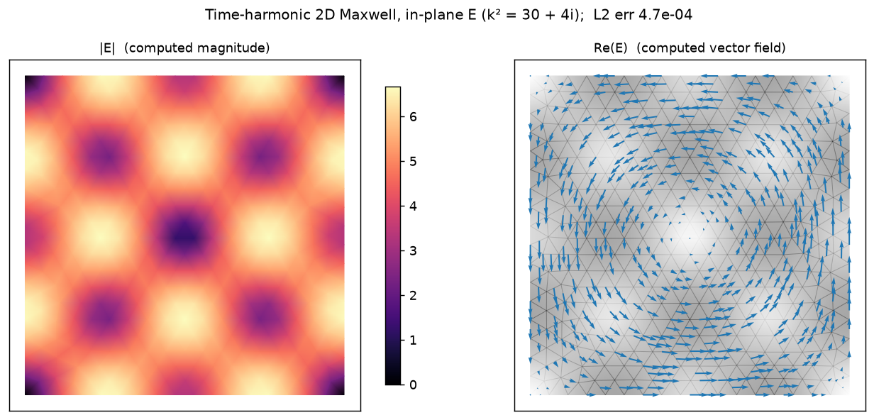
Left: \(|E| = \sqrt{|E_x|^2 + |E_y|^2}\) (computed). Right: the computed \(\mathrm{Re}(E)\) as a vector field — the rotational, divergence-free structure of a curl eigenmode. Both panels are the actual finite-element solution, nothing painted in.

What to notice

• Verified, not asserted: a manufactured divergence-free \(E\) with \(\mathrm{Re}(E)\neq\mathrm{Im}(E)\) and a genuinely complex \(k^2 = 30 + 4i\) (so the real and imaginary parts truly couple). At P2 the recovered field matches the closed-form \(E\) to \(L^2\) relative error \(\approx 5\times10^{-4}\).
• Generality by reuse: complex lowers onto the coupled-multifield path, so it inherits linear, nonlinear and transient for free — and the same trace expression drives a PINN.
• Honest scope: this uses nodal Lagrange elements with grad–div stabilisation (the right tool for a smooth field); general Maxwell with reentrant corners wants Nédélec edge elements.

Full script

"""11 - Time-harmonic 2D Maxwell (in-plane vector E field) with a genuine complex FEM field.

Frequency-domain Maxwell for the in-plane electric field ``E = (Ex, Ey)`` (TE polarisation) is the
**curl-curl** equation

    curl(curl E) - k^2 E = J ,     k^2 = omega^2 * mu * eps   (complex in a lossy medium),

with ``E`` complex-valued. jno exposes this directly: ``d.fem_symbols(..., complex=True)`` returns a
**complex** trial/test, so the weak form is written once with ordinary complex algebra (``*`` is the
complex product, ``1j``, ``.real``/``.imag``). Under the hood a complex field is carried as **two
coupled real fields** ``(E_r, E_i)`` and ``jno.fem`` lowers ``weak.real`` onto the coupled multifield
real system it already assembles -- the same machine behind the two-temperature / Stokes examples. No
separate "complex solver": ``1j`` is just the imaginary unit, the tracer carries the rest.

Two practical points for a *nodal* (Lagrange) discretisation of curl-curl:
  * the 2-D scalar curl is ``curl F = dFy/dx - dFx/dy`` -- written ``F.x[1] - F.y[0]`` (grad-then-index,
    since the backend differentiates the trial, not a component of it);
  * nodal elements need a **grad-div penalty** ``+ s * div(E) div(v)`` to kill the spurious curl
    kernel; it is consistent here because the exact field is divergence-free (so the penalty vanishes
    at the solution). With it, P1 converges ~O(h^2) and P2 is essentially exact.

Verification (no hand-waving): a manufactured divergence-free ``E`` with **Re(E) != Im(E)** and a
genuinely complex ``k^2`` -- curl(curl E_r)=2*pi^2 E_r, curl(curl E_i)=8*pi^2 E_i -- so the forcing is
``J = curl(curl E) - k^2 E`` in closed form. The script recovers it to a tight tolerance and renders
the *computed* field (no invented structure).
"""

import os

os.environ["MPLBACKEND"] = "Agg"

import jax

jax.config.update("jax_enable_x64", True)  # the coupled real system is float64

from pathlib import Path  # noqa: E402

import matplotlib.pyplot as plt  # noqa: E402
import matplotlib.tri as mtri  # noqa: E402
import numpy as np  # noqa: E402
from shapely.geometry import box  # noqa: E402

import jno  # noqa: E402

pi, sin, cos = np.pi, jno.np.sin, jno.np.cos
KR, KI = 30.0, 4.0  # k^2 = 30 + 4i  (non-resonant, lossy -> complex, non-singular)
k2 = KR + 1j * KI  # the complex coefficient, written as a plain Python complex

# manufactured divergence-free fields: E_r is a curl-eigenfield (eig 2*pi^2), E_i a higher mode (8*pi^2)
E_r = lambda X, Y: (pi * sin(pi * X) * cos(pi * Y), -pi * cos(pi * X) * sin(pi * Y))  # noqa: E731
E_i = lambda X, Y: (2 * pi * sin(2 * pi * X) * cos(2 * pi * Y), -2 * pi * cos(2 * pi * X) * sin(2 * pi * Y))  # noqa: E731

d = jno.domain(box(0.0, 0.0, 1.0, 1.0), mesh_size=0.06)
E, v = d.fem_symbols(value_shape=(2,), names=("E", "v"), order=2, complex=True)  # a P2 COMPLEX vector field + its test
xi, yi, _ = d.variable("interior", split=True)
xb, yb, _ = d.variable("boundary", split=True)
Eb, vb = E.bind(x=xi, y=yi), v.bind(x=xi, y=yi)

curl = lambda F: F.x[1] - F.y[0]  # dFy/dx - dFx/dy  # noqa: E731
div = lambda F: F.x[0] + F.y[1]  # noqa: E731
s = KR  # grad-div penalty weight (consistent: exact E is divergence-free)

exr, eyr = E_r(xi, yi)
exi, eyi = E_i(xi, yi)
# J = curl(curl E) - k^2 E, as complex data: J_r = (2pi^2 - kr) E_r + ki E_i ; J_i = (8pi^2 - kr) E_i - ki E_r
jxr, jyr = (2 * pi**2 - KR) * exr + KI * exi, (2 * pi**2 - KR) * eyr + KI * eyi
jxi, jyi = (8 * pi**2 - KR) * exi - KI * exr, (8 * pi**2 - KR) * eyi - KI * eyr
Jx, Jy = jno.complex(jxr, jxi), jno.complex(jyr, jyi)  # complex forcing components (re + 1j*im)

# ONE complex weak form; `.real` lowers it onto the coupled (E_r, E_i) real system.
weak = curl(Eb) * curl(vb) + s * div(Eb) * div(vb) - k2 * Eb.dot(vb) - (Jx * vb[0] + Jy * vb[1])
brx, bry = E_r(xb, yb)
bix, biy = E_i(xb, yb)  # E = exact on the wall (per-component: a coordinate-dependent vector BC is not yet one term)
fem = jno.fem(
    [
        weak.real,
        E.real(xb, yb)[0] - brx,
        E.real(xb, yb)[1] - bry,
        E.imag(xb, yb)[0] - bix,
        E.imag(xb, yb)[1] - biy,
    ],
    quad_degree=6,
)

A = jno.np.asarray(fem.A.todense()) if hasattr(fem.A, "todense") else jno.np.asarray(fem.A)
sol = np.asarray(np.linalg.solve(np.asarray(A), np.asarray(fem.b).reshape(-1)))
off = np.asarray(fem.problem.offset)
pts = np.asarray(fem.problem.mesh[0].points)
n = int(off[1])
E_re = sol[:n].reshape(-1, 2)  # computed Re(E) = (Ex_r, Ey_r) at every node
E_im = sol[n:].reshape(-1, 2)  # computed Im(E)

px, py = pts[:, 0], pts[:, 1]  # the manufactured reference, in plain numpy (E_r/E_i use jno.np for the trace)
ex_re = np.stack([pi * np.sin(pi * px) * np.cos(pi * py), -pi * np.cos(pi * px) * np.sin(pi * py)], axis=1)
ex_im = np.stack(
    [2 * pi * np.sin(2 * pi * px) * np.cos(2 * pi * py), -2 * pi * np.cos(2 * pi * px) * np.sin(2 * pi * py)], axis=1
)
rel = float(np.linalg.norm(np.concatenate([E_re - ex_re, E_im - ex_im])) / np.linalg.norm(np.concatenate([ex_re, ex_im])))
print("\n2D vector Maxwell (curl-curl, complex k^2) via a complex=True FEM field")
print(f"  4 real DOF/node, {fem.dofs} DOFs total;  L2 rel error vs manufactured E: {rel:.2e}")
assert rel < 2e-3, f"manufactured Maxwell not recovered: {rel:.2e}"

# ---- render the actual computed field (|E| and the Re(E) vectors) -- no invented structure ----
tris = np.asarray(fem.domain.built_mesh.cells_dict["triangle"])
triang = mtri.Triangulation(pts[:, 0], pts[:, 1], tris)
Emag = np.sqrt((E_re**2 + E_im**2).sum(1))  # |E| = sqrt(|Ex|^2 + |Ey|^2)
fig, ax = plt.subplots(1, 2, figsize=(11, 4.6))
tpc = ax[0].tripcolor(triang, Emag, cmap="magma", shading="gouraud")
fig.colorbar(tpc, ax=ax[0], shrink=0.85)
ax[0].set_title("|E|  (computed magnitude)", fontsize=10)
step = max(1, len(pts) // 400)
ax[1].tripcolor(triang, Emag, cmap="Greys", shading="gouraud", alpha=0.35)
ax[1].quiver(pts[::step, 0], pts[::step, 1], E_re[::step, 0], E_re[::step, 1], color="C0", scale=60, width=0.004)
ax[1].set_title("Re(E)  (computed vector field)", fontsize=10)
for a in ax:
    a.set_aspect("equal")
    a.set_xticks([])
    a.set_yticks([])
fig.suptitle(f"Time-harmonic 2D Maxwell, in-plane E (k² = {KR:g} + {KI:g}i);  L2 err {rel:.1e}", fontsize=11)
fig.tight_layout()
fig.savefig(Path(__file__).parents[2] / "assets" / "maxwell_2d_vector.png", dpi=130, bbox_inches="tight")