Adaptive mesh refinement (L-shape re-entrant corner)

Download .py All tutorials

The Laplace solution on the L-shape carries the classic \(r^{2/3}\) re-entrant-corner singularity. With Dirichlet data equal to the exact singular mode \(u = r^{2/3}\sin(2\varphi/3)\) about the corner \((0.5,0.5)\), \(u\) is harmonic — so all the discretization error comes from resolving that one corner. This tutorial resolves it two ways on the same problem, measured by the energy-norm error \(E-E_\text{ref}\) with \(E=\tfrac12\int|\nabla u_h|^2\) and \(E_\text{ref}\) from a fine mesh:

• h-adaptivity — add elements at the corner (the DOF count grows).
• differentiable r-adaptivity — relocate a fixed set of nodes down the energy gradient, computed through the differentiable solve (the DOF count is fixed).

The left panel jumps at each discrete remesh — new elements, more DOFs. The right panel flows continuously: the same nodes slide toward the corner, connectivity and DOF count unchanged.

Both live in the adapt= slot

h-adaptivity is one call. FEM.solve(adapt=jno.solve.remesh(...=)) runs the whole classical loop internally — solve → Zienkiewicz–Zhu estimate → Dörfler mark → local mmg remesh — then rebinds the FEM and mutates the domain to the final adapted mesh, recording each round on fem.adapt_history:

sol = fem.solve(adapt=jno.solve.remesh(theta=0.6, max_iters=4, refine_factor=1.7))   # ADD elements

r-adaptivity is the same slot with relocate=True. First make the interior vertices trainable: .trainable() on a spatial coordinate turns that region's mesh vertices into a design variable, so the assembler routes them into the element geometry and fem.solve() becomes differentiable in the node positions — the keystone \(\partial(\texttt{fem.solve})/\partial X\). The driver then moves them down the FE-energy gradient with a backtracking mesh-validity line search:

xm, ym, _ = d.variable("mov", where=interior, split=True)
xm.trainable(name="ix")            # literal, per component — x and y are separate coordinates
ym.trainable(name="iy")
...
sol = fem.solve(adapt=jno.solve.relocate(max_iters=60, lr=3e-3))         # RELOCATE nodes

No new DOFs, fixed connectivity, one JAX graph — no remeshing. The boundary is left fixed, so the L-shape itself never changes; only its interior nodes move. If relocate=True and no coordinate is tagged .trainable(), it fails loud.

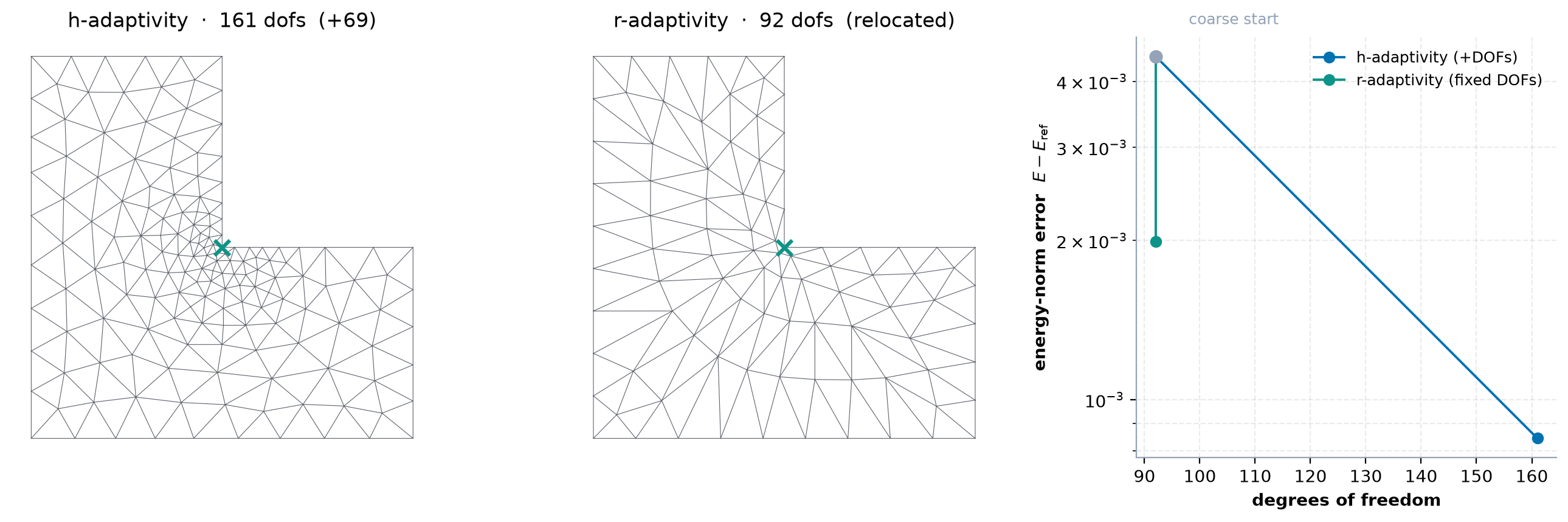
The result

From a 92-DOF coarse start (error \(4.5\times10^{-3}\)): h-adaptivity reaches \(8.4\times10^{-4}\) at 161 DOFs (+69, 81 % lower); r-adaptivity reaches \(2.0\times10^{-3}\) at the same 92 DOFs (55 % lower). h-adaptivity buys accuracy with DOFs; r-adaptivity buys it by moving the DOFs you already have.

What to notice

• The h-estimator is Zienkiewicz–Zhu — an inexpensive recovered-gradient indicator; Dörfler bulk-marking then selects the smallest set of elements carrying a fixed fraction of the total error. The remesh is a discrete, non-differentiable outer loop.
• The r-objective is the FE energy, minimized through the solve. Because the assembly geometry is pure JAX in the node coordinates, \(\partial(\texttt{fem.solve})/\partial X\) flows through the existing differentiable solve — the mechanism behind differentiable r-adaptivity (cf. G-Adaptivity, ICML 2025).
• Mesh validity is step control, not a loss term. The relocation checks \(\det J>0\) on the joint step and backtracks; a mesh-tangling barrier folded into the loss overshoots the huge near-corner gradients before it can react. Validity belongs in the line search, so the driver hand-rolls backtracking.
• The re-entrant corner is pinned for both mechanisms — h-adaptivity via mmg set_corners, r-adaptivity by leaving the boundary fixed — so the singularity stays put and the benchmark is honest.
• relocate=True composes across modes — linear, nonlinear, transient, periodic, vector and complex problems all relocate (the energy objective sums over every field block); only complex-transient is not yet supported, and it fails loud.

Full script

r"""Two ways to resolve the L-shape reentrant-corner singularity — **h-adaptivity** (add elements) and
**differentiable r-adaptivity** (relocate a *fixed* set of nodes), on the same problem, side by side.

    -lap u = 0  on the L-shape,  Dirichlet = the exact singular mode  u = r^(2/3) sin(2 phi / 3)
    about the reentrant corner (0.5, 0.5).

``u`` is harmonic, so all the discretization error is the ``r^(2/3)`` corner singularity, measured here by
the **energy-norm error** ``E - E_ref`` with ``E = ½∫|∇u_h|²`` and ``E_ref`` from a fine mesh.

* **h-adaptivity** — ``fem.solve(adapt=jno.solve.remesh(...=))`` runs the whole classical loop internally
  (``solve -> Zienkiewicz-Zhu estimate -> Dörfler mark -> local remesh``): it **adds** elements at the
  corner. The remesh is a discrete, non-differentiable outer loop.
* **r-adaptivity** — make the interior vertex coordinates trainable (``x.trainable()``) and move them down
  the energy gradient, computed *through the differentiable solve* (``∂(fem.solve())/∂X``, the keystone).
  It **relocates** a fixed node set — no new DOFs, fixed connectivity, one JAX graph, no remeshing.

Run::

    JAX_PLATFORMS=cpu pixi run -e fem python docs/tutorial_examples/08_fem_and_varpinns/adaptive_l_shape.py
"""

from __future__ import annotations

import os

import numpy as np

os.environ.setdefault("JAX_PLATFORMS", "cpu")  # small FEM solves; keep off the GPU

import jax  # noqa: E402

jax.config.update("jax_enable_x64", True)

import jax.numpy as jnp  # noqa: E402

import jno  # noqa: E402
import jno.jnp_ops as J  # noqa: E402

L_SHAPE = [(0, 0), (1.0, 0), (1.0, 0.5), (0.5, 0.5), (0.5, 1.0), (0, 1.0)]  # reentrant corner at (0.5, 0.5)
MARGIN = 0.025  # keep the movable interior nodes off the boundary (incl. the two notch edges)


def _mod(a, m):  # jno.np has no `mod`; build it from `floor` (works on trace symbols and numpy)
    return a - m * J.floor(a / m)


def u_singular(x, y, xp, mod):
    X, Y = x - 0.5, y - 0.5
    r = xp.sqrt(X * X + Y * Y)
    phi = mod(mod(xp.arctan2(Y, X), 2.0 * np.pi) - np.pi / 2.0, 2.0 * np.pi)  # 3*pi/2-wide material wedge
    return (r ** (2.0 / 3.0)) * xp.sin(2.0 / 3.0 * phi)


def _interior(x, y):
    """True interior L-shape vertices: inside the material, off the outer box and the two notch edges."""
    inside = ~((x > 0.5) & (y > 0.5))
    off_box = (x > MARGIN) & (x < 1 - MARGIN) & (y > MARGIN) & (y < 1 - MARGIN)
    off_notch = ~(((jnp.abs(x - 0.5) < MARGIN) & (y > 0.5 - MARGIN)) | ((jnp.abs(y - 0.5) < MARGIN) & (x > 0.5 - MARGIN)))
    return inside & off_box & off_notch


def build(size, movable=False):
    d = jno.Shape.polygon(L_SHAPE, size=size).domain()
    u, phi = d.fem_symbols()
    xi, yi, _ = d.variable("interior", split=True)
    xb, yb, _ = d.variable("boundary", split=True)
    if movable:
        # ---- the r-adaptivity API ----------------------------------------------------------------------
        # `.trainable()` on a spatial coordinate turns that region's mesh VERTICES into a design variable:
        # the assembler routes them into the element geometry, so `fem.solve()` becomes differentiable in
        # the node positions. Literal, per component (x and y are separate). Must be called BEFORE jno.fem.
        # The boundary is left fixed, so the L-shape itself never changes — only its interior nodes move.
        xm, ym, _ = d.variable("mov", where=_interior, split=True)
        xm.trainable(name="ix")
        ym.trainable(name="iy")
        # -------------------------------------------------------------------------------------------------
    ui, vi = u.bind(x=xi, y=yi), phi.bind(x=xi, y=yi)
    fem = jno.fem([ui.x * vi.x + ui.y * vi.y, u(xb, yb) - u_singular(xb, yb, J, _mod)])
    return d, fem


def dirichlet_energy(pts, sol, cells):
    """``½∫|∇u_h|²`` for a P1 field, straight from the vertices + nodal values — differentiable in BOTH
    (so it works as the r-adaptivity objective ``∂E/∂X`` through the solve). The FE energy is bounded below
    by the true energy and falls as the mesh resolves the corner, so minimizing it is the energy-norm-error
    goal (Ciarlet, *The Finite Element Method for Elliptic Problems*, 1978)."""
    v = pts[cells]
    s = sol[cells]
    x0, x1, x2 = v[:, 0, 0], v[:, 1, 0], v[:, 2, 0]
    y0, y1, y2 = v[:, 0, 1], v[:, 1, 1], v[:, 2, 1]
    detJ = (x1 - x0) * (y2 - y0) - (x2 - x0) * (y1 - y0)
    gx = (s[:, 0] * (y1 - y2) + s[:, 1] * (y2 - y0) + s[:, 2] * (y0 - y1)) / detJ
    gy = (s[:, 0] * (x2 - x1) + s[:, 1] * (x0 - x2) + s[:, 2] * (x1 - x0)) / detJ
    return 0.25 * jnp.sum((gx * gx + gy * gy) * jnp.abs(detJ))


def _solve(fem):
    A, b = fem.A, fem.b
    Ad = jnp.asarray(A.todense() if hasattr(A, "todense") else A)
    return jnp.linalg.solve(Ad, jnp.asarray(b).reshape(-1))


def _min_detj(pts, cells):
    v = pts[cells]
    a, b = v[:, 1] - v[:, 0], v[:, 2] - v[:, 0]
    return float(np.min(a[:, 0] * b[:, 1] - a[:, 1] * b[:, 0]))


# --- reference energy (fine mesh) and a common coarse starting mesh ---------------------------------------
d_ref, fem_ref = build(0.03)
E_REF = float(
    dirichlet_energy(
        jnp.asarray(np.asarray(d_ref.mesh.points)[:, :2]), _solve(fem_ref), jnp.asarray(d_ref.mesh.cells_dict["triangle"])
    )
)

# (1) h-adaptivity — ADD elements: one call runs the whole solve→estimate→mark→remesh loop and returns the
#     solution on the final adapted mesh (`d_h`/`fem_h` now refer to it).
d_h, fem_h = build(0.12)
n0 = len(d_h.mesh.points)
pts0, tris0 = np.asarray(d_h.mesh.points)[:, :2], np.asarray(d_h.mesh.cells_dict["triangle"])
E0 = float(dirichlet_energy(jnp.asarray(pts0), _solve(fem_h), jnp.asarray(tris0)))
sol_h = np.asarray(fem_h.solve(adapt=jno.solve.remesh(theta=0.6, max_iters=4, refine_factor=1.7))).reshape(-1)
pts_h, tris_h = np.asarray(d_h.mesh.points)[:, :2], np.asarray(d_h.mesh.cells_dict["triangle"])
E_h = float(dirichlet_energy(jnp.asarray(pts_h), jnp.asarray(sol_h), jnp.asarray(tris_h)))
n_h = len(sol_h)

# (2) r-adaptivity — RELOCATE a fixed node set: the SAME `adapt=` slot with `relocate=True`. The interior
#     vertices were tagged `.trainable()` in build(); the driver moves them (no new DOFs) and returns the solve.
d_r, fem_r = build(0.12, movable=True)
pts_r0 = np.asarray(d_r.mesh.points)[:, :2].copy()  # coarse start, for the animation
sol_r = np.asarray(fem_r.solve(adapt=jno.solve.relocate(max_iters=60, lr=3e-3))).reshape(-1)
pts_r, tris_r = np.asarray(d_r.mesh.points)[:, :2], np.asarray(d_r.mesh.cells_dict["triangle"])
E_r = float(dirichlet_energy(jnp.asarray(pts_r), jnp.asarray(sol_r), jnp.asarray(tris_r)))

print(f"energy-norm error  (E - E_ref),  E_ref = {E_REF:.4f}")
print(f"  coarse start   : {E0 - E_REF:.3e}   ({n0} dofs)")
print(
    f"  h-adaptivity   : {E_h - E_REF:.3e}   ({n_h} dofs, +{n_h - n0})   {100 * (1 - (E_h - E_REF) / (E0 - E_REF)):.0f}% lower"
)
print(f"  r-adaptivity   : {E_r - E_REF:.3e}   ({n0} dofs, +0)   {100 * (1 - (E_r - E_REF) / (E0 - E_REF)):.0f}% lower")

# h-adaptivity adds DOFs and lowers the error; r-adaptivity lowers it at FIXED DOFs, without tangling.
assert n_h > n0, "h-adaptivity should add DOFs at the corner"
assert E_h - E_REF < 0.4 * (E0 - E_REF), "h-adaptivity should sharply cut the energy error"
assert E_r - E_REF < 0.75 * (E0 - E_REF), "r-adaptivity should cut the energy error at fixed DOFs"
assert _min_detj(pts_r, tris_r) > 0, "r-adaptivity must not tangle the mesh"