Topology Optimisation on a Deformable Mesh

Download .py All tutorials

The classic SIMP cantilever — minimise compliance at a \(40\%\) volume fraction — except the mesh is a design variable too. The optimiser drives one vector \([\rho, d_x, d_y]\): an element density per triangle, plus the position of every interior node. The boundary is resolved by moving nodes onto it rather than by refining until the staircase stops mattering. This is the method of K. Jung and D.-N. Kim, Density-based topology optimization using a deformable mesh, Computers & Structures (2025), doi:10.1016/j.compstruc.2025.107879.

Three design variables, one optimiser

Densities live on elements (space="P0", one dof per triangle, their eq. 12). Nodal coordinates become parameters through .trainable(), which must be called before jno.fem(...) because the assembler reads the coordinate registry when it builds. Both kinds are discovered and stepped together by jno.core:

xm, ym, _ = d.variable("mv", where=interior, split=True)
xm.trainable(name="mesh_x"), ym.trainable(name="mesh_y")
_r, s = d.fem_symbols(space="P0", names=("r", "s"))
rho = jno.np.parameter(s, name="rho")
rho.optimizer(jno.optimizers.mma(move=0.15, lower=1e-3, upper=1.0))

jno.optimizers.mma is the Method of Moving Asymptotes (Svanberg 1987) — a sentinel optimiser, detected by solve() rather than being a plain optax transform, because it needs the individual constraint values and gradients that a scalar-loss transform never sees.

The constraints that make it legal

Free nodal movement will happily invert an element, so the mesh needs its own constraints — minimum interior angle, and maximum/minimum element volume (their eq. 24/26/28), aggregated with a \(p=50\) norm. d.cell_angles() and d.cell_volume() are trace nodes, so they are differentiable in the nodal coordinates, which is exactly what makes them usable as constraints — and being nodes, they are written as the arithmetic they are:

g_ang = ((2*jnp.pi - d.cell_angles()) / (2*jnp.pi - THETA_MIN)).reshape(-1).pnorm(50.0, normalize=True)
crux = jno.core([compliance, jno.le(volume, 1.0), jno.le(g_ang, 1.0), ...], domain=...)

jno.le marks a constraint the optimiser handles but does not add to the loss. Without it every constraint doubles as a soft penalty and fights MMA's own dual handling. normalize=True matters more than it looks: summing \(N\) terms at \(p=50\) overshoots the true maximum by a factor growing with \(N\), so an unnormalised aggregate reads as a violation from iteration 0 and freezes MMA before it takes a step. (Measured at \(+7.7\%\) on a coarser version of this problem, and it grows with the mesh.)

Manufacturability: the patch filter and perimeter control

Two separate levers, and they enter the pipeline in two different ways.

The patch filter (their eq. 17–19) replaces the usual density filter. It drives to zero exactly those elements whose neighbourhood makes the layout unbuildable — a one-node connection, or a lone dense element — and leaves everything else alone. It is non-local, so it cannot live inside the weak form, where the kernel sees one element at a time. It goes in as a reparameterisation:

patch = d.patch_filter()
rho.constrain(lambda r: jnp.where(pmask, 1.0, patch(r)))   # physics sees the PHYSICAL density

Perimeter control is the feature-scale knob. \(P\) sums the smoothed density jump across every interior edge (Haber, Jog & Bendsøe 1996); holding it under a target \(P^\*\) forbids the optimiser from buying stiffness with ever-finer members. It enters as an interior penalty, \(R=-\beta\log(P^\*-P)\), not as a jno.le constraint:

terms.append(jno.fn(lambda rr, bb: bb[0] * rr, [rho.perimeter(zeta=0.1).log_barrier(PSTAR), beta_p]))
callbacks.append(jno.optimizers.geometric_decay(beta_p, 0.997, start=BETA, minimum=BETA_MIN))

log_barrier extends the logarithm quadratically once \(P\) comes within \(\tau\) of the bound. This is not a detail: a plain log(max(P* - P, eps)) is constant above the bound, so its gradient there is exactly zero and the barrier silently stops doing anything — the failure mode is a satisfied-looking run whose perimeter sits far above target.

Perimeter is a global budget, and converged designs exploit that

A design can meet \(P^\*\) exactly and still be locally serrated, paying for a spike here with flatness elsewhere. Measured on a converged 3-D bracket with the barrier active and satisfied, the angle between adjacent surface facets had a median of \(33.5^\circ\), a 99th percentile of \(88.9^\circ\), and \(27\%\) of adjacent pairs above \(60^\circ\) — a surface nobody would machine, scoring as well on eq. (38) as a smooth one would. Neither cheap lever fixes it: un-throttling node migration un-pinned the nodes (\(27.3\% \to 6.2\%\) sitting at their move bound) and moved the roughness only \(33.5^\circ \to 32.0^\circ\), while tightening \(P^\*\) from 44 to 31 bought \(26.9^\circ\) at \(91\%\) worse compliance. Both also collapsed the volume constraint, to \(V=0.705\) and \(0.635\) against the baseline's \(0.998\).

rho.curvature(zeta=0.1) is the local measure the perimeter is not — the discrete bending energy of a triangle mesh (Grinspun, Hirani, Desbrun & Schröder, Discrete Shells, SCA 2003, §3), summed over pairs of interior facets sharing a ridge (a mesh vertex in 2-D, a mesh edge in 3-D). Each pair costs \(|\Delta_i||\Delta_j|(1-\cos\theta_{ij})\) in the sharp limit, so it is zero unless both facets carry boundary and then grows with the angle between them. It is orientation-free (facet normal and density jump flip signs together), non-negative by construction, and exactly zero both on a flat boundary and where there is no boundary at all.

Add it as a penalty rather than a constraint — MMA already has the volume and the geometric bounds to trade against, and that trade is where the volume collapses:

S = rho.curvature(zeta=0.1)
terms.append(WEIGHT * S)          # weight in compliance units; see the scale note below

A weight needs a scale and the design cannot supply one, because at iteration 0 the density is uniform and the bending is exactly zero. Take it from the mesh instead — what a single flat cut already costs, purely from its own faceting. That floor is real (an unstructured interface zig-zags between tetrahedra rather than lying in the plane it approximates, the same reason a straight bar's perimeter measures above its length) but it does not track refinement: measured \(50.7\) at \(h=0.5\) against \(52.4\) at \(h=0.35\), across a \(2.6\times\) change in tet count. So WEIGHT = w / S_ref keeps \(w\) comparable across meshes.

The comparison that shows the two functionals are genuinely different: under a monotone staircase boundary the perimeter telescopes to one horizontal unit per column plus the total rise, whatever route the staircase takes. Three designs of identical volume and identical perimeter — \(14.0000\) to every decimal place — score \(S = 2\), \(10\), \(12\), exactly their right-angle counts.

	one big step	five small ones	a staircase
perimeter \(P\)	\(14.0000\)	\(14.0000\)	\(14.0000\)
bending \(S\)	\(2\)	\(10\)	\(12\)

In 3-D the separation is milder and the honest number is the ratio between the functionals: a square corrugation at fixed volume raises \(P\) by \(1.59\times\) and \(S\) by \(1.90\times\); scrambling the same material raises \(P\) by \(14.6\times\) and \(S\) by \(48.2\times\). So bending is about \(1.2\times\) sharper on a fold and \(3.3\times\) sharper on noise — worth its own term, and not a replacement for perimeter control.

Under a deformable mesh the term is also differentiable in the node coordinates, which is half the point: it gives node migration a reason to align the boundary rather than merely shorten it.

The patch filter has a size limit, and it is lower than it looks

Eq. (18) is a geometric mean over \(N-2\) factors, and a mean dilutes a single outlier by \(1/N\). So the criterion's discriminating power is set by how many elements meet at the vertex. Measured on the shipped kernel (tests/test_patch_filter_scaling.py), with \(f_\text{solid}=1\) throughout:

\(N\)	lone dense element	one-node connection	uniform grey	hinge / solid
5 (3-D edge fan, \(6T/E\))	0.100	0.013	0.831	0.01
6 (2-D vertex, \(3T/V\))	0.178	0.038	0.842	0.04
8	0.316	0.112	0.853	0.11
12	0.501	0.755	0.862	0.76
27 (3-D vertex, \(4T/V\))	0.758	0.845	0.870	0.85

At the size a 2-D triangulation actually produces (\(N\approx6\)) the filter separates a defect from a grey patch by a factor of \(4.7\), which is what makes it work. By \(N=12\) three-quarters of that is gone, and a valence-12 vertex is not exotic on an unstructured mesh — so on a badly graded 2-D mesh the filter quietly weakens where the patches are largest. At \(N\approx27\), the size of a tetrahedral vertex patch, a hinge sits within \(3\%\) of uniform grey and nothing downstream can act on it; SIMP cannot finish the job either, since \(0.758^3 = 0.44\) of solid against \(0.006\) for the \(0.178\) of a six-element patch.

This is a property of any mean — a density-weighted geometric mean with exponent \(1/\sum\rho\) behaves the same — so it is not recoverable by reweighting. The practical consequences: a 3-D vertex criterion needs an order statistic rather than eq. (18), while a 3-D edge fan (\(6T/E\approx5.2\)) sits in the regime where the formula is at its strongest — it discriminates a hinge three times more sharply than the 2-D vertex patch it was designed for — and so transfers verbatim. This is the extension Jung, Yun & Kim leave open in their §2.3.2.

The objective is an integral

Compliance is the strain energy C = a(u,u) = ∫ σ(u):ε(u) dΩ, and it is written as exactly that — the same bilinear form the weak statement is built from, integrated at the solution:

eps = lambda w: symgrad(w, [xi, yi])
a   = lambda p, q: LAM*trace(p)*trace(q) + 2*MU*inner(p, q, n_contract=2)
E   = lambda r: EMIN + r**penal_p * (E0 - EMIN)

fem        = jno.fem([E(rho) * a(eps(u), eps(phi)), ...])
compliance = (E(rho) * a(eps(u), eps(u))).integrate(fem)
rho_e      = rho.reshape(-1)                                 # (n_cells, 1) -> (n_cells,); see below
volume     = (rho_e * cellv).sum / (VOLFRAC * cellv.sum)     # NOT an .integrate(fem) — see below

reshape(-1) is load-bearing, and omitting it fails silently

A P0 parameter evaluates to (n_cells, 1) while cell_volume() is (n_cells,), so rho * cellv broadcasts to an (n_cells, n_cells) outer product whose .sum is n_cells times too large. Nothing raises — it is a valid shape. The volume constraint then reads as satisfied at a design carrying almost no material, and compliance climbs instead of falling. Measured on a 128-cell 2-D problem: the constraint reported 1.0000 while the design it accepted had a volume fraction of 0.0078, and compliance ran to 4.5e4 against the 18.6 the flattened form reaches on the same 12 iterations.

.integrate(fem) inherits the quadrature the operator was assembled with, so this equals f·u exactly rather than to within a quadrature error nothing reports. The fem is named because it is the one thing the expression cannot supply: a trial symbol carries its basis, but not the solution values, the assembly quadrature, or which system to differentiate through. Every functional over one fem shares a single solve.

Use it where quadrature is actually needed. rho.integrate(fem) gives the right volume, but ρ is piecewise constant, so ∫ρ dΩ is exactly Σ ρ_k |K| — and routing it through the functional runs a full element map, plus its backward pass, to compute a weighted sum. Measured on this problem, at 400 iterations: compliance as an integral costs 84 s against 80 s for the frozen-load-vector version, about 4 %; adding the volume as an integral too pushed the same run past 7 minutes. The rule that falls out is not "avoid the functional" but "use it for what has an integrand" — an energy density needs the basis and the quadrature, a per-element sum does not.

This matters past tidiness. The objective used to be a dot product against a load vector evaluated outside the trace, and the volume a lambda over cell_volume() — so every new objective needed its own reduction over the DOF vector. As integrals, a stress constraint (((sigma_vm/SIG_Y)**p).integrate(fem)), a compliant mechanism's output displacement, and multiple load cases are all the same one construct.

Pick the solver — in 3-D it is most of the run

integrate(fem, solver=...) selects the backend for the solve every functional over that fem shares. It is the single biggest lever on a design loop, because the solve runs once forward and once adjoint per iteration on a sparsity that never changes — relocation moves nodes, not connectivity — so a backend that caches its symbolic analysis pays only the numeric re-factorisation:

C = (E(rho) * a(eps(u), eps(u))).integrate(fem, solver=jno.solve.lu(backend="pardiso"))

Measured on the 3-D cantilever, per design iteration, against the default:

tetrahedra	default	`backend="pardiso"`	speed-up
2,847	620 ms	335 ms	1.9x
8,802	2,115 ms	665 ms	3.2x
14,063	4,014 ms	810 ms	5.0x

The margin grows with the mesh because the two scale differently on this operator — the default's SuperLU costs \(O(n^{1.9})\) against PARDISO's \(O(n^{1.55})\) — so it is worth most exactly where it is needed. Two reasons the headroom is there: the stiffness is symmetric positive definite (to \(5.6\times10^{-17}\)) while the default throws a general LU at it, and the default re-runs its symbolic analysis every call.

backend="pardiso" is not usable with the patch filter yet

Those timings are measured on plain SIMP with a volume constraint — no rho.constrain(d.patch_filter()). With the patch filter in place the PARDISO backend aborts the process with a glibc double free or corruption, at every mesh size tried. Controlled A/B, with no CUDA device visible: pardiso alone works, the filter alone works under the default backend, the pair dies. It is not the GPU, not MKL threading, not pure_callback concurrency, not the adjoint/transpose path, and not cache eviction — each was checked and ruled out; the cause is still open.

So on a design run today the default backend is the one that works, and the speed-up above is available only to problems that do not reparameterise their density. That is what bounds a 30-minute run to roughly 14k elements at ~350 iterations rather than 65k.

An iterative solver is not the answer here, which is worth stating because it is the usual advice at this size: smoothed-aggregation AMG with elasticity's near-nullspace converges fine (residual \(10^{-11}\)) but needs 103–145 CG iterations against the \(10^3\) SIMP contrast, landing at 244–1250 ms — an order of magnitude worse than the direct factorisation. Contrast is what makes a SIMP system hard for a multigrid hierarchy, and it is exactly what topology optimisation creates.

Every sensitivity is automatic

The paper hand-derives \(\partial C/\partial\rho\) and \(\partial C/\partial d_{x_i} = -\sum_{j\in S_i}(u^j)^{\mathsf T}(\partial k^j_0/\partial d_{x_i})u^j\) — the derivative of each element stiffness with respect to its three nodes' coordinates — across two pages. None of that is written here. fem.solve() is a differentiable trace node and trainable coordinates are ordinary parameters, so MMA gets its gradients from AD.

Always reanalyse — and calibrate the reanalysis

An optimiser that moves nodes can lower compliance either by improving the structure or by distorting elements until they under-integrate strain energy, and it cannot tell those apart from the inside. The check is to transfer the converged density to a clean, undistorted mesh and re-solve:

rho_ref = d.transfer_cell_field(rho_f, d_ref, points=pts_f, outside=1e-3)   # points= -> deformed source

A raw gap is not by itself a distortion measurement — the reference mesh is finer, and a coarse mesh is over-stiff on its own. The script therefore also runs a control carrying no design and no distortion at all (uniform density on both meshes). Here that control shows only \(+0.8\%\), so the reference mesh is genuinely converged and the excess is attributable to the moved nodes. Skipping this control is how a load-application bug or a plain refinement effect gets reported as a method result.

The reanalysis script that produces the numbers below

Kept separate from the optimisation run because it is a check on the result, not part of producing it. It is a CLI tool, not a runnable example — it takes the converged design and re-solves it on a clean mesh:

python reanalysis.py --design <design>.npz [--h-fine 0.5] [--threshold 0.5]

The optimisation script above does not currently write that .npz

So the two do not connect out of the box: you have to save rho_f yourself at the end of the run before this script can consume it. The numbers in the table below were produced that way.

"""Reanalysis: does the optimised design report its own stiffness honestly?

The optimiser moves nodes AND densities, so it can lower compliance either by improving the
structure or by distorting elements until they under-integrate strain energy and report a
stiffness they do not have. Those are indistinguishable from inside the run. The test that
separates them (Jung, Yun & Kim 2026, Fig. 7c-d) is to take the converged design, freeze it as a
binary layout, and re-solve it on a FRESH, UNDISTORTED mesh:

    C_design      the design's own number, on its own deformed mesh
    C_reanalysis  the same layout on a clean fine mesh

If they agree the reported stiffness is real. If C_reanalysis is much higher, the run was farming
discretisation error. The paper measures +17.6 % for the conventional element and -0.5 % with
E-FEM; that gap is what the enrichment exists to close.
"""

import argparse
import logging

import jax

jax.config.update("jax_enable_x64", True)

import jax.numpy as jnp  # noqa: E402
import numpy as np  # noqa: E402
from matplotlib.tri import TrapezoidMapTriFinder, Triangulation  # noqa: E402

import jno  # noqa: E402

inner, symgrad, trace = jno.np.inner, jno.np.symgrad, jno.np.trace

p = argparse.ArgumentParser()
p.add_argument("--design", required=True, help="path to the .npz design field to re-analyse")
p.add_argument("--h-fine", type=float, default=0.5, help="reanalysis mesh size")
p.add_argument("--threshold", type=float, default=0.5)
args = p.parse_args()
logging.disable(logging.INFO)

L, H = 60.0, 30.0
E0, EMIN, NU, VOLFRAC = 1.0, 1e-9, 0.3, 0.4
LAM, MU = E0 * NU / (1 - NU**2), E0 / (2 * (1 + NU))
TOL = 1e-6 * L


def build(size, trainable=False):
    """The SAME weak form as the optimisation run: clamped left, unit traction on the right."""
    d = jno.shape.rect(0, 0, L, H, size=size).domain()
    if trainable:
        xm, ym, _ = d.variable("mv", where=lambda x, y: (x > TOL) & (x < L - TOL) & (y > TOL) & (y < H - TOL), split=True)
        xm.trainable(name="mesh_x"), ym.trainable(name="mesh_y")
    u, phi = d.fem_symbols(value_shape=(2,))
    _r, s = d.fem_symbols(space="P0", names=("r", "s"))
    xi, yi, _ = d.variable("interior", split=True)
    xl, yl, _ = d.variable("left", split=True)
    xr, yr, _ = d.variable("right", split=True)
    rho = jno.np.parameter(s, name="rho")
    rho.dtype(jnp.float64)
    eu, ep = symgrad(u, [xi, yi]), symgrad(phi, [xi, yi])
    fem = jno.fem(
        [
            (EMIN + rho**3.0 * (E0 - EMIN)) * (LAM * trace(eu) * trace(ep) + 2 * MU * inner(eu, ep, n_contract=2)),
            u(xl, yl) - (0.0, 0.0),
            -1.0 * inner(jnp.array([0.0, -1.0 / H]), phi.bind(x=xr, y=yr), n_contract=1),
        ],
        quad_degree=2,
    )
    return d, fem


def compliance(fem, args_dict):
    """C = f . u, from the assembled system — no optimiser, no trace."""
    a, b = fem.operator.evaluate(args_dict)
    a_d = np.asarray(jnp.asarray(a.todense()), dtype=np.float64)
    f = np.asarray(jnp.asarray(b).reshape(-1), dtype=np.float64)
    u = np.linalg.solve(a_d, f)
    return float(f @ u), u


z = np.load(args.design)
pts_def, cells_def, rho_e = z["pts"], z["cells"], z["rho_e"]
solid = rho_e > args.threshold
binary = np.where(solid, 1.0, 1e-3)
print(f"design: {cells_def.shape[0]} elements, {int(solid.sum())} solid ({solid.mean():.3f} by count), reported C = 77.974")

# --- 1. the design's own number, on its own deformed mesh, made BINARY --------------------------
d_def, fem_def = build(1.0, trainable=True)
specs = d_def._trainable_coords
ids = np.asarray(specs[0]["ids"], dtype=int)
coord_args = {sp["name"]: jnp.asarray(pts_def[ids, int(sp["axis"])]) for sp in specs}
assert np.asarray(d_def._cells_p1()).shape == cells_def.shape, "mesh mismatch — regenerate"

c_grey, _ = compliance(fem_def, {"rho": jnp.asarray(rho_e), **coord_args})
c_bin_def, _ = compliance(fem_def, {"rho": jnp.asarray(binary), **coord_args})
print(f"on the deformed mesh:   grey C = {c_grey:.4f}   binary C = {c_bin_def:.4f}")

# --- 2. the same layout on a fresh undistorted mesh ---------------------------------------------
d_new, fem_new = build(args.h_fine)
cells_new = np.asarray(d_new._cells_p1())
pts_new = np.asarray(d_new.mesh.points)[:, :2]
cen_new = pts_new[cells_new].mean(axis=1)

# Which deformed element does each new element's centroid fall in? Exact point-in-triangle via
# matplotlib's trapezoid map; -1 means outside the deformed mesh (impossible here, same domain).
finder = TrapezoidMapTriFinder(Triangulation(pts_def[:, 0], pts_def[:, 1], cells_def))
owner = finder(cen_new[:, 0], cen_new[:, 1])
outside = int((owner < 0).sum())
rho_new = np.where(owner >= 0, rho_e[np.maximum(owner, 0)], 1e-3)
print(
    f"reanalysis mesh: {cells_new.shape[0]} elements ({outside} centroids outside), "
    f"solid fraction {float((rho_new > 0.5).mean()):.3f}"
)

c_re, _ = compliance(fem_new, {"rho": jnp.asarray(rho_new)})
rho_new_bin = np.where(owner >= 0, binary[np.maximum(owner, 0)], 1e-3)
c_re_bin, _ = compliance(fem_new, {"rho": jnp.asarray(rho_new_bin)})

# --- verdict ------------------------------------------------------------------------------------
gap = 100.0 * (c_re - c_grey) / c_grey
gap_bin = 100.0 * (c_re_bin - c_bin_def) / c_bin_def
print("\n" + "=" * 68)
print("  DENSITY TRANSFERRED AS-IS -- isolates discretisation from thresholding")
print(f"  C reported by the design, on its deformed mesh   : {c_grey:10.4f}")
print(f"  C of the same density field on a clean fine mesh : {c_re:10.4f}")
print(f"  the design over-reports its stiffness by         : {gap:+9.2f} %")
print("  --")
print(f"  thresholded at {args.threshold}: deformed {c_bin_def:.3e} -> clean {c_re_bin:.3e} ({gap_bin:+.2f} %)")
print("  (paper: +17.6 % conventional, -0.5 % with E-FEM)")
print("=" * 68)

Result

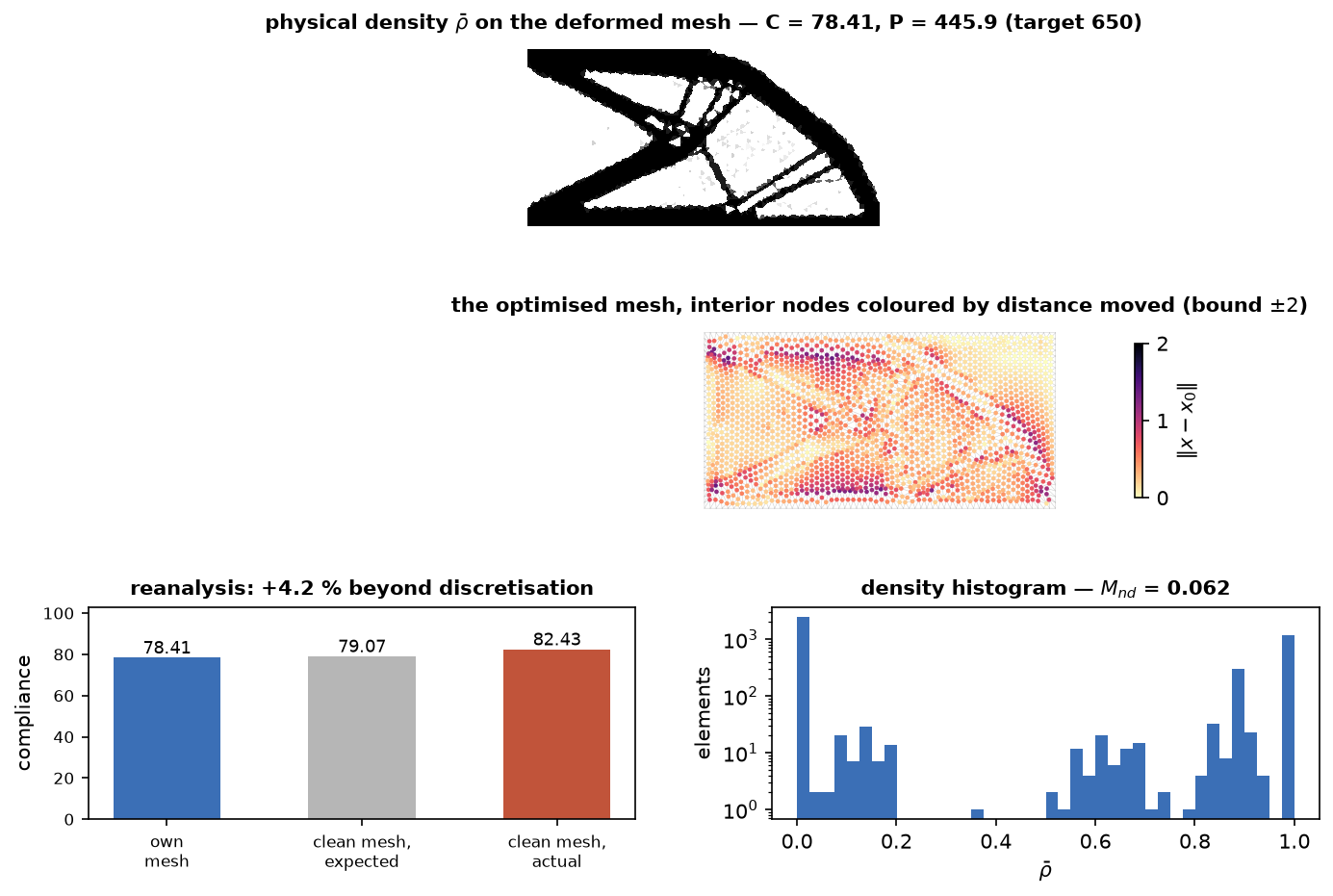
4,226 elements, 4,408 dofs, 400 iterations, ~3 min on CPU:

quantity	value
compliance, own deformed mesh	\(78.41\)
compliance, clean mesh (16,828 elements)	\(82.43\) (raw gap \(+5.1\%\))
control, uniform density, no distortion	\(661.28 \to 666.87\) (\(+0.8\%\) discretisation)
over-report attributable to the moved nodes	\(+4.2\%\) (but see below)
perimeter \(P\)	\(445.9\) against target \(P^\*=650\)
volume fraction / \(M_{nd}\) / inverted elements	\(0.4000\) / \(0.062\) / \(0\)

Which of these numbers are reproducible

Not all of them, and the difference matters more than any single value. Four runs of this script — one before the objective was rewritten as an integral, two after, differing only in the Python and JAX build they ran on, and run D on a later jNO (parameters float64 since #123), which is the one in the table and the figure above:

	run A	run B	run C	run D
compliance	\(78.45\)	\(78.33\)	\(78.64\)	\(78.41\)
volume fraction	\(0.400\)	\(0.3998\)	\(0.3999\)	\(0.4000\)
\(M_{nd}\)	\(0.075\)	\(0.066\)	\(0.071\)	\(0.062\)
perimeter \(P\)	\(587.2\)	\(504.1\)	\(530.7\)	\(445.9\)
over-report	\(+13.6\%\)	\(+5.4\%\)	\(+10.2\%\)	\(+4.2\%\)

Compliance and volume fraction are stable to a fraction of a percent — they are what the problem actually pins down. The perimeter and the reanalysis gap are not: they span \(446\)–\(587\) and \(+4.2\)–\(+13.6\%\). Runs B and C are the same source code, so this is not the rewrite; it is the problem. It is non-convex, and MMA's asymptote update is history-dependent with a branch in it — a variable that just reversed direction has its asymptotes pulled in, one moving steadily has them pushed out — so a change in the last bit of a floating-point operation flips that test for some variable, and the trajectories separate from there into different local optima.

(It is not the SIMP continuation, which would be the obvious suspect. Measured on this configuration: penal stays at \(3.0\) and the continuation fires zero times in 400 iterations — see the note below.)

The practical consequence: quote the over-report as a range, "\(+4\) to \(+14\%\)", and not to three figures, and treat a single run's perimeter as one sample rather than a measurement. (\(C = f\cdot u\) and \(C = \int \sigma(u){:}\varepsilon(u)\,d\Omega\) agree in value and in gradient analytically — both reduce to \(-u^{\mathsf T}(\partial K/\partial\rho)u\) — so the rewrite changes the arithmetic path, not the objective.)

Perimeter control earns its place, though not in every column. Running the same script with PSTAR = 0.0 gives \(P=849.2\), \(C=80.23\), \(M_{nd}=0.127\) and an over-report of \(+21.6\%\) (measured on the previous spelling of the objective and not re-run since). Against the spread above, the binariness separates cleanly — \(M_{nd}\) \(0.127\) uncontrolled against \(0.062\)–\(0.075\) controlled — and the perimeter obviously does. The over-report comparison does not: \(+21.6\%\) against a controlled range of \(+4.2\)–\(+13.6\%\) is a difference of the same size as the run-to-run scatter, so one uncontrolled run is not enough to claim it. What survives is the binariness, and the mechanism behind it: a design held to a length scale has fewer fine features to farm discretisation error with.

Do not read the accompanying drop in compliance (\(80.23 \to 78.45\)) as perimeter control being free. Without a length-scale restriction the continuum problem is not well posed — that is exactly why Ambrosio & Buttazzo introduced the perimeter constraint and Haber, Jog & Bendsøe implemented it — and numerically the unregularised run fragments instead of converging. On the companion half-MBB problem the uncontrolled run measurably fails to settle: doubling the iteration budget moved compliance the wrong way, \(209.9 \to 224.5\), with perimeter rising \(1274 \to 1302\). An uncontrolled baseline is therefore a poor reference point, and the honest claim here is that perimeter control makes the problem tractable enough to converge — not that it costs nothing.

For scale, the paper reports \(+17.6\%\) for conventional elements on its own cantilever and closes the gap to \(-0.5\%\) with the interpolation-cover enrichment of its 2026 follow-up (Computers & Structures 331 (2026) 108403), which this tutorial does not implement.

What to notice

.trainable() on coordinates must precede jno.fem(...).
space="P0" gives one design value per element; jno.np.parameter sizes it from the symbol.
jno.le(...) = constraint the optimiser sees but does not descend; rho.constrain(...) = reparameterisation the physics sees. They are not interchangeable — MMA only gets a multiplier for the former.
A near-point traction must be applied over a span that the node predicate actually covers: y < SPAN drops the facet ending exactly at SPAN, which silently scales the load by \((\mathrm{SPAN}-h)/\mathrm{SPAN}\).
x64 is on — the \(p=50\) aggregation needs the exponent range.

Full script

"""Topology optimisation on a deformable mesh: density AND nodal positions as design variables.

The classic SIMP cantilever, but the mesh is a design variable too. The optimiser drives one
vector [rho, d_x, d_y] -- an element density per triangle, plus the position of every interior
node -- so the boundary is resolved by *moving nodes onto it* rather than by refining until the
staircase is small. This is the method of

  K. Jung and D.-N. Kim, "Density-based topology optimization using a deformable mesh",
  Computers & Structures (2025), doi:10.1016/j.compstruc.2025.107879.
  Perimeter control follows R.B. Haber, C.S. Jog and M.P. Bendsoe, "A new approach to
  variable-topology shape design using a constraint on perimeter", Struct. Optim. 11 (1996) 1-12.

Three pieces make it work, and each is one line here:

  * `space="P0"`         one design value per ELEMENT (their eq. 12), not per node
  * `d.patch_filter()`   their eq. (17)-(19): a physical density that drives one-node
                         connections and lone dense elements to zero. It replaces the usual
                         density filter, and being NON-LOCAL it enters as a reparameterisation
                         (`rho.constrain`), not as a term in the weak form
  * `jno.le(...)`        geometric constraints (min angle, max/min element volume) that keep the
                         mesh valid while its nodes move -- their eq. (24)/(26)/(28)

**Every sensitivity is automatic.** The paper hand-derives dC/drho and dC/dX -- the latter needs
the derivative of each element stiffness with respect to its three nodes' coordinates -- across
two pages. Here `fem.solve()` is a differentiable trace node and trainable coordinates are
ordinary parameters, so MMA gets its gradients from AD and none of that is written down.

The run ends with a **reanalysis**, which is not optional: an optimiser that moves nodes can
lower compliance either by improving the structure or by distorting elements until they
under-integrate strain energy, and it cannot tell those apart from the inside. Transferring the
converged density to a clean, undistorted mesh and re-solving is the check that separates them.
"""

import jax

jax.config.update("jax_enable_x64", True)  # geometric constraints at p=50 need the exponent range

import jax.numpy as jnp  # noqa: E402
import numpy as np  # noqa: E402
import optax  # noqa: E402

import jno  # noqa: E402

inner, symgrad, trace = jno.np.inner, jno.np.symgrad, jno.np.trace

L, H, h = 60.0, 30.0, 1.0  # domain and target edge length (the paper's constants below assume h=1)
E0, EMIN, NU, PENAL, VOLFRAC = 1.0, 1e-9, 0.3, 3.0, 0.4
LAM, MU = E0 * NU / (1 - NU**2), E0 / (2 * (1 + NU))  # plane stress
THETA_MIN, PNORM = np.deg2rad(20.0), 50.0  # min interior angle; p-norm aggregation exponent
V0MAX, V0MIN = 0.75 * h**2, 0.05 * h**2  # element-volume bounds, scaled from edge length 1
MOVE_BOUND, SPAN, TOL, ITERS = 2.0 * h, 2.0 * h, 1e-6 * L, 400
PSTAR, BETA, GAMMA, BETA_MIN = 650.0, 2e-4, 0.997, 1e-4  # perimeter target and barrier schedule

d = jno.shape.rect(0, 0, L, H, size=h).domain()
pts0 = np.asarray(d.mesh.points)[:, :2]
cells = np.asarray(d._cells_p1())

# --- design variables 2 and 3: the interior nodal coordinates --------------------------------
# Nodes on the outer boundary stay put (they define the domain); everything inside may move,
# bounded by +/-MOVE_BOUND from where it started. `.trainable()` must precede `jno.fem(...)`,
# which reads the coordinate registry when it builds.
interior = lambda x, y: (x > TOL) & (x < L - TOL) & (y > TOL) & (y < H - TOL)  # noqa: E731
xm, ym, _ = d.variable("mv", where=interior, split=True)
xm.trainable(name="mesh_x"), ym.trainable(name="mesh_y")
ids = np.asarray(d._trainable_coords[0]["ids"], dtype=int)
for spec in d._trainable_coords:
    x0 = pts0[ids, int(spec["axis"])]
    spec["expr"].optimizer(
        jno.optimizers.mma(move=0.02, lower=x0 - MOVE_BOUND, upper=x0 + MOVE_BOUND, move_gamma=0.9985, move_min=0.001)
    )

# --- design variable 1: one density per element ----------------------------------------------
u, phi = d.fem_symbols(value_shape=(2,))  # P1 vector displacement
_r, s = d.fem_symbols(space="P0", names=("r", "s"))  # P0 scalar -> one dof per triangle
xi, yi, _ = d.variable("interior", split=True)
xl, yl, _ = d.variable("left", split=True)  # clamped root
xt, yt, _ = d.variable("tip", where=lambda x, y: (x > L - TOL) & (y < SPAN + TOL), split=True)

rho = jno.np.parameter(s, name="rho")
rho.dtype(jnp.float64)
rho.initialize(jax.nn.initializers.constant(VOLFRAC))
rho.optimizer(jno.optimizers.mma(move=0.15, lower=1e-3, upper=1.0, move_gamma=0.9985, move_min=0.0075))

# `penal` is a runtime parameter so the continuation can raise it without triggering a recompile.
penal_p = jno.np.parameter((1,), name="penal")
penal_p.dtype(jnp.float64)
penal_p.initialize(lambda k, sh, dtype=None: jnp.full(sh, PENAL))
penal_p.optimizer(optax.sgd(1.0))

# Solid, non-designable material where the load is applied. Without it the optimiser empties the
# loaded elements and the compliance then measures that artefact rather than the structure.
cen0 = pts0[cells].mean(axis=1)
pmask = jnp.asarray((cen0[:, 0] > L - SPAN) & (cen0[:, 1] < SPAN))
patch = d.patch_filter()  # eq. (17)-(19)
rho.constrain(lambda r: jnp.where(pmask, 1.0, patch(r)))  # physics sees the PHYSICAL density

# --- the elasticity problem -------------------------------------------------------------------
# Bind the notation once so the weak form and the objective below read like the equations, and so
# they demonstrably share one bilinear form rather than being two hand-typed copies of it.
eps = lambda w: symgrad(w, [xi, yi])  # noqa: E731
a = lambda p, q: LAM * trace(p) * trace(q) + 2 * MU * inner(p, q, n_contract=2)  # noqa: E731  sigma(p):q
E = lambda r: EMIN + r**penal_p * (E0 - EMIN)  # noqa: E731  -- SIMP: E(rho) = Emin + rho^p (E0 - Emin)

fem = jno.fem(
    [
        E(rho) * a(eps(u), eps(phi)),
        u(xl, yl) - (0.0, 0.0),  # clamped root
        -1.0 * inner(jnp.array([0.0, -1.0 / SPAN]), phi.bind(x=xt, y=yt), n_contract=1),
    ],
    quad_degree=2,
)

# --- the objective and the constraints, as the integrals they are ------------------------------
# Compliance is the strain energy C = a(u,u) = ∫ sigma(u):eps(u) dOmega -- the SAME form the weak
# statement above is built from, integrated at the solution. `.integrate(fem)` inherits the
# quadrature the operator was assembled with, so this equals f.u exactly rather than to within a
# quadrature error; naming the `fem` supplies what the expression cannot (which solution, which
# system to differentiate through), and every functional over one `fem` shares a single solve.
cellv, angles = d.cell_volume(), d.cell_angles()  # differentiable in the nodal coordinates
# A P0 parameter evaluates to (n_cells, 1) while `cell_volume()` is (n_cells,), so pairing them
# without this flatten broadcasts to an (n_cells, n_cells) OUTER PRODUCT whose sum is n_cells times
# too large -- silently, since it is a valid shape. Flatten once, here.
rho_e = rho.reshape(-1)
compliance = (E(rho) * a(eps(u), eps(u))).integrate(fem).name("C")
# The volume needs no quadrature: rho is piecewise constant, so ∫rho dOmega is exactly sum(rho_k |K|)
# and `cell_volume()` is already a node differentiable in the moving mesh. Routing it through the FEM
# functional would run a full element map to compute a weighted sum -- same answer, far more work.
volume = ((rho_e * cellv).sum / (VOLFRAC * cellv.sum)).name("V")
g_ang = (((2 * jnp.pi - angles) / (2 * jnp.pi - THETA_MIN)).reshape(-1).name("g1")).pnorm(
    PNORM, normalize=True
)  # eq. (24): no interior angle below theta_min
g_vmx = ((cellv / ((2.0 - rho_e) * V0MAX)).name("g2")).pnorm(PNORM, normalize=True)  # eq. (26): no element grows past V0max
g_vmn = (((2 * V0MAX - cellv) / (2 * V0MAX - V0MIN)).name("g3")).pnorm(
    PNORM, normalize=True
)  # eq. (28): none collapses below V0min

# --- perimeter control: the feature-scale lever, eq. (38)-(41) ---------------------------------
# P sums the density jump across every interior edge (Haber, Jog & Bendsoe 1996), smoothed by
# zeta. Holding it under a target P* forbids the optimiser from buying stiffness with ever-finer
# members, so it is the manufacturability knob: lower P* -> fewer, thicker bars.
#
# It enters as an INTERIOR PENALTY, R = -beta * log(P* - P), not as a `jno.le` constraint --
# that is the paper's eq. (39)-(40). `log_barrier` extends the log quadratically once P gets
# within tau of the bound: a plain log(max(P*-P, eps)) goes CONSTANT above the bound, so its
# gradient is exactly zero there and the barrier silently stops doing anything.
# `beta` decays geometrically (eq. 41) so the barrier stops distorting the converged optimum.
perim = rho.perimeter(zeta=0.1)
beta_p = jno.np.parameter((1,), name="beta")
beta_p.dtype(jnp.float64)
beta_p.initialize(lambda k, sh, dtype=None: jnp.full(sh, BETA))
beta_p.optimizer(optax.sgd(1.0))

# `jno.le` marks a constraint the optimiser handles but does NOT add to the loss -- without it
# every constraint doubles as a soft penalty and fights MMA's own dual handling.
terms = [compliance]
# `watch=0` points the continuation at the COMPLIANCE: under a decaying barrier the total loss
# keeps drifting, so a convergence test on the total would never fire.
callbacks = [jno.optimizers.simp_continuation(penal_p, rho, physical=patch, every=25, watch=0)]
if PSTAR > 0:
    terms.append((beta_p[0] * perim.log_barrier(PSTAR)).name("R"))
    callbacks.append(jno.optimizers.geometric_decay(beta_p, GAMMA, start=BETA, minimum=BETA_MIN))
terms += [jno.le(volume, 1.0), jno.le(g_ang, 1.0), jno.le(g_vmx, 1.0), jno.le(g_vmn, 1.0)]

crux = jno.core(terms, domain=jno.domain.from_array({"_": np.zeros((1, 1))}))
crux.solve(ITERS, callbacks=callbacks)

rho_f = np.asarray(crux.eval([rho])).reshape(-1)  # PHYSICAL density (constrain applies first)
pts_f = pts0.copy()
for spec in d._trainable_coords:
    pts_f[ids, int(spec["axis"])] = np.asarray(crux.eval([spec["expr"]])).reshape(-1)
C = float(np.asarray(crux.eval([compliance])).reshape(-1)[0])
P = float(np.asarray(crux.eval([perim])).reshape(-1)[0])  # the smoothed perimeter, eq. (38)

# --- the honesty check: re-solve the SAME design on a clean, undistorted mesh -------------------
d_ref = jno.shape.rect(0, 0, L, H, size=h / 2).domain()  # fresh, twice as fine, undeformed
rho_ref = d.transfer_cell_field(rho_f, d_ref, points=pts_f, outside=1e-3)  # `points=` -> deformed source
u2, phi2 = d_ref.fem_symbols(value_shape=(2,))
_r2, s2 = d_ref.fem_symbols(space="P0", names=("r2", "s2"))
xi2, yi2, _ = d_ref.variable("interior", split=True)
xl2, yl2, _ = d_ref.variable("left", split=True)
xt2, yt2, _ = d_ref.variable("tip", where=lambda x, y: (x > L - TOL) & (y < SPAN + TOL), split=True)
rho2 = jno.np.parameter(s2, name="rho2")
rho2.dtype(jnp.float64)
eu2, ep2 = symgrad(u2, [xi2, yi2]), symgrad(phi2, [xi2, yi2])
fem_ref = jno.fem(
    [
        (EMIN + rho2**PENAL * (E0 - EMIN)) * (LAM * trace(eu2) * trace(ep2) + 2 * MU * inner(eu2, ep2, n_contract=2)),
        u2(xl2, yl2) - (0.0, 0.0),
        -1.0 * inner(jnp.array([0.0, -1.0 / SPAN]), phi2.bind(x=xt2, y=yt2), n_contract=1),
    ],
    quad_degree=2,
)
import scipy.sparse as sp  # noqa: E402
import scipy.sparse.linalg as spla  # noqa: E402


def solve_C(operator, args):  # compliance from an assembled system, by sparse-direct factorisation
    A, b = operator.evaluate(args)
    f = np.asarray(jnp.asarray(b).reshape(-1), dtype=np.float64)
    i = np.asarray(A.indices)
    K = sp.csr_matrix((np.asarray(A.data, dtype=np.float64), (i[:, 0], i[:, 1])), shape=(f.size, f.size))
    return float(f @ spla.spsolve(K.tocsc(), f))


C_ref = solve_C(fem_ref.operator, {"rho2": jnp.asarray(np.asarray(rho_ref).reshape(-1))})

# A raw reanalysis gap is NOT a distortion measurement: the reference mesh is finer, and a coarse
# mesh is over-stiff on its own. Calibrate that away with a control carrying no design and no
# distortion at all -- a uniform density on the undeformed coarse mesh and on the clean fine one.
# Whatever gap THAT shows is pure discretisation, and only the excess above it is attributable to
# the moved nodes. (A first-order correction: compliance error does not factorise exactly.)
n_c, n_f = cells.shape[0], d_ref._cells_p1().shape[0]
coord0 = {sp["name"]: jnp.asarray(pts0[ids, int(sp["axis"])]) for sp in d._trainable_coords}  # UNdeformed
C_u_coarse = solve_C(fem.operator, {"rho": jnp.full(n_c, VOLFRAC), "penal": jnp.asarray([PENAL]), **coord0})
C_u_fine = solve_C(fem_ref.operator, {"rho2": jnp.full(n_f, VOLFRAC)})
discretisation = C_u_fine / C_u_coarse  # the coarse mesh's intrinsic over-stiffness
excess = (C_ref / C) / discretisation - 1.0  # what the node movement bought that was not real

vol = (
    np.abs(np.linalg.det(np.stack([pts_f[cells][:, 1] - pts_f[cells][:, 0], pts_f[cells][:, 2] - pts_f[cells][:, 0]], -1)))
    / 2
)
print(
    f"\nTopology optimisation: {n_c} elements, {fem.dofs} dofs, {ITERS} iterations"
    f"\n  compliance (own deformed mesh)          = {C:9.4f}"
    f"\n  compliance (clean mesh, {n_f} elements) = {C_ref:9.4f}   raw gap {100 * (C_ref - C) / C:+.1f} %"
    f"\n  control, uniform density, no distortion = {C_u_coarse:9.4f} -> {C_u_fine:9.4f}"
    f"   ({100 * (discretisation - 1):+.1f} % is pure discretisation)"
    f"\n  => stiffness over-report attributable to the moved nodes: {100 * excess:+.1f} %"
    f"\n  perimeter P = {P:.3f}"
    + (f" against target P* = {PSTAR:.1f}" if PSTAR > 0 else " (uncontrolled)")
    + f"\n  volume fraction = {np.sum(rho_f * vol) / np.sum(vol):.4f}   "
    f"M_nd = {4 * np.mean(rho_f * (1 - rho_f)):.4f}   inverted elements = {int((vol <= 0).sum())}"
)
assert PSTAR <= 0 or P < PSTAR  # the barrier kept the perimeter under its bound
assert np.sum(rho_f * vol) / np.sum(vol) < VOLFRAC * 1.05  # volume constraint respected
assert int((vol <= 0).sum()) == 0  # the geometric constraints kept every element valid