Poisson 2D (FDM)

Download .py All tutorials

The strong-form counterpart of the Poisson FEM primer: \(-\Delta u = f\) on the unit square with \(u = 0\) on the boundary, solved through jno.fdm. Instead of a weak form, the strong residual is collocated at the mesh nodes with finite-difference stencils.

Result

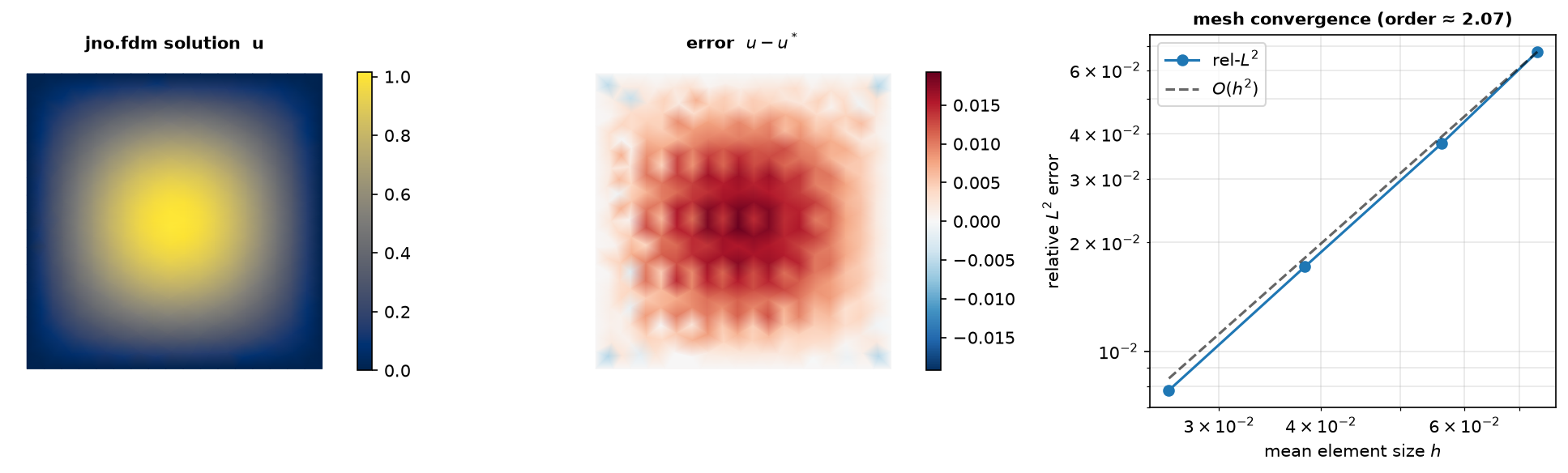
The jno.fdm field matches the manufactured \(u^\* = \sin(\pi x)\sin(\pi y)\) to rel-\(L^2 \approx 1.7\times10^{-2}\) on this mesh, and re-solving at four mesh sizes shows the error falling at second order (fitted slope \(\approx 2.07\), right) — the expected rate for the finite-difference Laplacian.

The constraint list

u = domain.unknown() is a valued nodal field — the strong-form counterpart of fem_symbols(). Binding it gives the FD derivative views (ui.d2(x) is the finite-difference second derivative, no scheme= needed), and the Dirichlet condition is the term u(region) - g:

u  = d.unknown()
ui = u.bind(x=x, y=y)
f  = 2.0 * np.pi**2 * jnn.sin(np.pi * x) * jnn.sin(np.pi * y)
sol = jno.fdm([
    -ui.d2(x) - ui.d2(y) - f,   # -Delta u = f
    u(xb, yb) - 0.0,            # Dirichlet u = 0
]).solve()

What to notice

• One call, jno.fdm([...]), builds the strong-form system and .solve() returns the nodal field.
• The API mirrors jno.fem: domain.unknown() for the trial, .bind for derivatives, boundary conditions as terms in the same list.
• A nodal field's .d / .d2 default to finite differences — autodiff is meaningless on a discrete field, so no scheme= is needed (pass one to pick a different stencil).
• The solution is audited against the manufactured field \(u^\* = \sin(\pi x)\sin(\pi y)\) (rel-\(L^2 \approx 1.7\times10^{-2}\), the expected FD-discretization error on this mesh).

Full script

"""01 - 2D Poisson equation solved through ``jno.fdm`` (finite differences, strong form).

    -Delta u = f on the unit square, u = 0 on the boundary.
    Manufactured  u*(x, y) = sin(pi x) sin(pi y),   f = 2 pi^2 sin(pi x) sin(pi y).

``jno.fdm`` is the **strong-form sibling** of ``jno.fem``: author the PDE and its boundary
conditions as the *same* constraint list, with ``u = domain.unknown()`` (a valued nodal field, the
counterpart of ``fem_symbols()``). Instead of a weak form with test functions and quadrature, the
strong residual is collocated at the mesh nodes with finite-difference stencils -- so ``ui.d2(x)`` is
the FD second derivative (autodiff is meaningless on a discrete field, so FD is the default; no
``scheme=`` needed). The Dirichlet condition is the term ``u(region) - g``, exactly as in ``jno.fem``.
"""

import jax

jax.config.update("jax_enable_x64", True)  # the strong-form solve accumulates in float64

import numpy as np  # noqa: E402

import jno  # noqa: E402
import jno.jnp_ops as jnn  # noqa: E402

d = jno.Shape.rect(0.0, 0.0, 1.0, 1.0, size=0.06).domain()
x, y, _ = d.variable("interior", split=True)
xb, yb, _ = d.variable("boundary", split=True)
u = d.unknown()  # valued P1 nodal field (strong-form counterpart of fem_symbols())
ui = u.bind(x=x, y=y)  # bound view with .d / .d2 (FD by default)

f = 2.0 * np.pi**2 * jnn.sin(np.pi * x) * jnn.sin(np.pi * y)
sol = jno.fdm(
    [
        -ui.d2(x) - ui.d2(y) - f,  # -Delta u = f   (finite differences at the mesh nodes)
        u(xb, yb) - 0.0,  # Dirichlet u = 0 on the boundary
    ]
).solve()

p = np.asarray(d.mesh_connectivity["points"])[:, :2]  # the nodes the DOFs live on
exact = np.sin(np.pi * p[:, 0]) * np.sin(np.pi * p[:, 1])
rel_l2 = float(np.linalg.norm(np.asarray(sol).reshape(-1) - exact) / np.linalg.norm(exact))
print(f"\nPoisson via jno.fdm: nodes={p.shape[0]}  rel_L2={rel_l2:.3e}")
assert rel_l2 < 3e-2, f"relative L2 error too large: {rel_l2:.3e}"