Mixed Boundary Conditions (FDM)

Download .py All tutorials

Dirichlet, Neumann, and Robin conditions on the same problem — steady conduction on the unit square with the manufactured field \(u^\* = y^2\) (so \(-\Delta u = -2\)):

edge	condition
bottom (\(y=0\))	Dirichlet \(u = 0\)
top (\(y=1\))	Robin \(\partial_n u + (u - 3) = 0\)
left / right	Neumann \(\partial_n u = 0\) (insulated)

Result

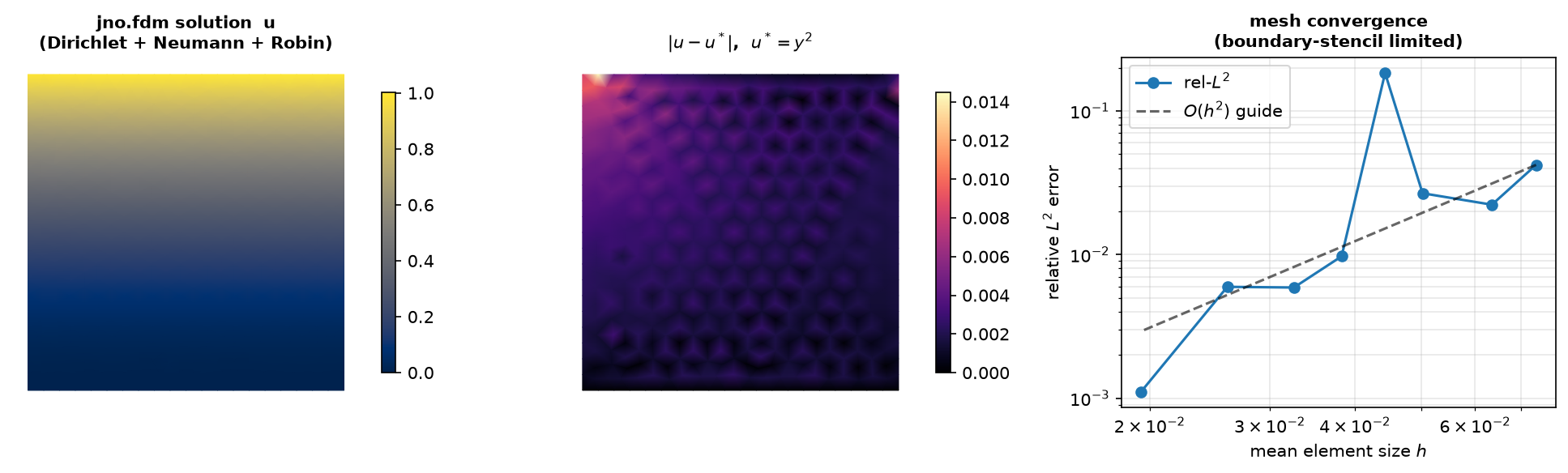
The recovered field matches \(u^\* = y^2\) to rel-\(L^2 \approx 5.7\times10^{-3}\) on the working mesh. Because the interior field is a quadratic (so the interior FD residual is essentially exact), the error lives almost entirely at the boundaries: the one-sided Neumann/Robin edge stencils and the corner PDE-fallback set the accuracy. Under refinement (right) the error trends down from \(\sim\!4\times10^{-2}\) to \(\sim\!10^{-3}\), but not at a clean \(O(h^2)\) rate — it is mesh-sensitive and scatters, as the boundary stencils are re-sampled by each unstructured mesh.

Flux conditions are written with the edge's own tags

Get the outward normal from domain.variable(region, normals=True), bind the field to the edge, and take its normal derivative. Any condition affine in \(\partial_n u\) works the same way — jno.fdm reads the coefficient of the normal derivative directly, so Neumann and Robin are the same mechanism:

nr = d.variable("right", normals=True)
ur = u.bind(x=xr, y=yr)          # field bound to the right edge

ur.d(nr) - 0.0                   # Neumann: du/dn = 0
ut.d(nt) + 1.0 * (ut - 3.0)      # Robin:   du/dn + (u - 3) = 0

What to notice

• Any mix of Dirichlet / Neumann / Robin on different edges composes in one list — no special BC objects.
• A flux condition binds the field to that edge (ur = u.bind(x=xr, y=yr)) and uses it for both the flux term and any value term, so the whole edge equation reads from one set of boundary tags.
• Corner nodes shared by two flux edges have no single outward normal, so they fall back to the interior PDE residual (give a corner a Dirichlet value if it needs anchoring).
• The recovered field matches \(u^\* = y^2\) to the FD-discretization accuracy (rel-\(L^2 \approx 5\times10^{-3}\)).

Full script

"""02 - Mixed boundary conditions through ``jno.fdm``: Dirichlet + Neumann + Robin at once.

Steady conduction on the unit square with the manufactured field ``u*(x, y) = y^2`` (so -Delta u = -2):

    * bottom (y = 0):  Dirichlet   u = 0
    * top    (y = 1):  Robin       du/dn + (u - 3) = 0     (at y=1: du/dn = 2, u = 1  ->  2 + (1-3) = 0)
    * left / right  :  Neumann     du/dn = 0               (insulated; u = y^2 is flat in x)

A flux boundary condition is written with **that edge's own tags** -- bind the field to the edge
(``ur = u.bind(x=xr, y=yr)``) and take its normal derivative ``ur.d(nr)`` against the outward normal
``nr = domain.variable(region, normals=True)``. Any condition **affine in** ``du/dn`` works the same
way: Neumann ``ur.d(n) - h``, Robin ``ur.d(n) + alpha*(u - u_inf)``, either sign -- ``jno.fdm`` reads
the coefficient of ``du/dn`` directly, no special BC objects. Corner nodes shared by two flux edges
fall back to the interior PDE residual.
"""

import jax

jax.config.update("jax_enable_x64", True)

import numpy as np  # noqa: E402

import jno  # noqa: E402

d = jno.Shape.rect(0.0, 0.0, 1.0, 1.0, size=0.05).domain()
x, y, _ = d.variable("interior", split=True)
xbo, ybo, _ = d.variable("bottom", split=True)
xl, yl, _ = d.variable("left", split=True)
xr, yr, _ = d.variable("right", split=True)
xt, yt, _ = d.variable("top", split=True)
nl = d.variable("left", normals=True)  # outward-normal Variables, one per edge
nr = d.variable("right", normals=True)
nt = d.variable("top", normals=True)

u = d.unknown()
ui = u.bind(x=x, y=y)  # interior view for the PDE
ul = u.bind(x=xl, y=yl)  # edge-bound views for the flux conditions
ur = u.bind(x=xr, y=yr)
ut = u.bind(x=xt, y=yt)

sol = jno.fdm(
    [
        -ui.d2(x) - ui.d2(y) + 2.0,  # -Delta u = -2   (manufactured u = y^2)
        u(xbo, ybo) - 0.0,  # Dirichlet: bottom held at 0
        ul.d(nl) - 0.0,  # Neumann: left insulated (du/dn = 0)
        ur.d(nr) - 0.0,  # Neumann: right insulated
        ut.d(nt) + 1.0 * (ut - 3.0),  # Robin: top convects to u_inf = 3 with alpha = 1
    ]
).solve()

p = np.asarray(d.mesh_connectivity["points"])[:, :2]
exact = p[:, 1] ** 2  # u = y^2
rel_l2 = float(np.linalg.norm(np.asarray(sol).reshape(-1) - exact) / np.linalg.norm(exact))
print(f"\nMixed Dirichlet+Neumann+Robin via jno.fdm: nodes={p.shape[0]}  rel_L2={rel_l2:.3e}")
assert rel_l2 < 5e-2, f"relative L2 error too large: {rel_l2:.3e}"