Bayesian inverse PINN: recover a PDE coefficient

Download .py Back to chapter

Inverse uncertainty quantification. A steady reaction–diffusion system -λ u''(x) + k u(x) = f(x) on the unit line with a known forcing f and an unknown reaction coefficient k. We observe the field u at noisy sensors and want the posterior over k — a value and an honest credible interval, not just a point estimate.

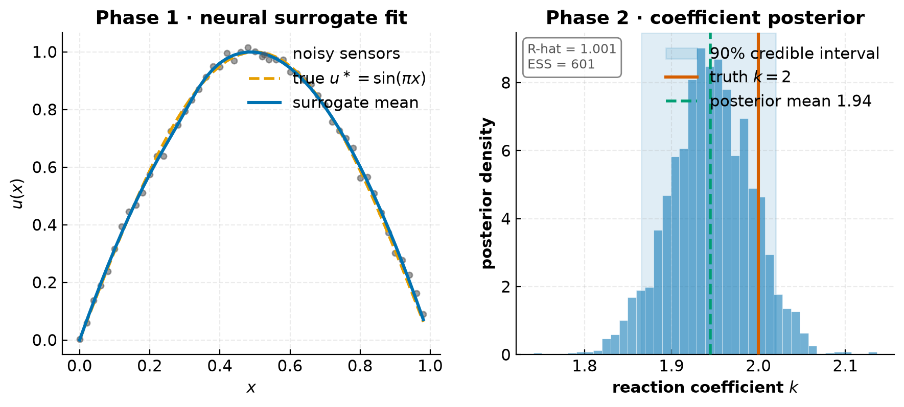
The two-stage recipe

Sampling the full ~1 000-weight network posterior on a stiff PINN loss is hard to calibrate. The robust pattern samples only the tractable unknown instead:

1. Fit a neural surrogate u_net to the noisy sensor data with optax (deterministic). Hard u·x·(1-x) factors impose the u(0)=u(1)=0 BCs.
2. u_net.freeze() turns the surrogate into a fixed forward map, so NUTS samples a well-defined, fixed-target posterior over the single scalar k through the physics residual -λ u'' + k u - f. A fixed target is what makes window adaptation well-defined and the posterior cheap and cleanly calibrated.

u_net.freeze()                                   # fixed forward map
k = jno.np.parameter((1,), name="k")
k.bayesian(blackjax.nuts, step_size=1e-2, warmup=300, keep=600,
           num_chains=4, init_jitter=0.5)        # 4 chains ⇒ a meaningful R-hat

uf = u_net(x) * x * (1 - x)
residual = (-LAMBDA * uf.dd(x) + k * uf - f_known) / SIGMA_PHYS
jno.core([residual.mse]).solve(900)              # recovers the posterior over k

What to notice

• The credible interval covers the truth. k = 1.94 ± 0.05, 90% CI [1.87, 2.02], which contains the true k = 2 — with R-hat ≈ 1.00 and ESS ≈ 600 across four chains confirming the chains mixed.
• sigma_phys budgets for model error, not just observation noise. A differentiated neural surrogate carries a small u'' bias; setting the physics likelihood scale to cover it is what keeps the posterior honest (truth inside the interval) rather than over-confident.
• Read the chain, not a point estimate. A narrow interval away from the truth would signal an over-tight sigma_phys or a poor surrogate; a very wide interval means the data and physics simply don't pin k down.

Reference

Yang, L., Meng, X., & Karniadakis, G. E. (2021). B-PINNs: Bayesian physics-informed neural networks for forward and inverse PDE problems with noisy data. Journal of Computational Physics, 425, 109913.

Script

"""01 — Bayesian inverse PINN: recover a PDE coefficient with calibrated UQ.

Governing physics (steady reaction-diffusion on the unit line, u(0)=u(1)=0):

    -lambda u''(x) + k u(x) = f(x),   lambda = 1 known,   k unknown.

We observe the field ``u`` at noisy sensors and know the forcing ``f``; the goal
is the *posterior* over the reaction coefficient ``k`` — a value **and** an honest
credible interval — not just a point estimate.

The robust two-stage recipe (the one the chapter index recommends):

  Phase 1 — fit a smooth neural **surrogate** ``u_net`` to the noisy sensor data
            (deterministic, optax).
  Phase 2 — ``u_net.freeze()`` turns the surrogate into a *fixed* forward map, so
            NUTS samples a well-defined, fixed-target posterior over ``k`` through
            the physics residual.  Sampling a single scalar (not the ~1k network
            weights) is what makes the posterior cleanly calibrated and cheap.

The likelihood scale ``sigma_phys`` budgets for **surrogate model error**, not just
observation noise — inflating it to cover the small bias a differentiated surrogate
introduces is what keeps the truth inside the credible interval (see the assert).
"""

from pathlib import Path

import blackjax
import foundax
import jax
import jax.numpy as jnp
import numpy as np
import optax

import jno

π = jno.np.pi

# ── Physical setup ────────────────────────────────────────────────────────────
LAMBDA = 1.0  # known diffusivity
K_TRUE = 2.0  # the reaction coefficient we will recover
SIGMA_U = 0.02  # sensor noise on the observed field u
SIGMA_PHYS = 0.05  # physics likelihood scale (obs noise + surrogate model error)

domain = jno.Path(0.0, 0.0).line_to(1.0, 0.0).curve(size=0.02).domain()
x, _ = domain.variable("interior")
x_np = np.asarray(domain.context["interior"]).reshape(-1, 1)

# Fixed noisy sensor observations of the true field u*(x) = sin(πx).
rng = np.random.default_rng(0)
u_obs = jnp.asarray(np.sin(π * x_np) + SIGMA_U * rng.normal(size=x_np.shape))

# The forcing is a *known* physical input; here it is the f that makes u*=sin(πx)
# the true solution:  f = -λ u*'' + k_true u* = (λπ² + k_true) sin(πx).
f_known = (LAMBDA * π**2 + K_TRUE) * jno.np.sin(π * x)

# ══ Phase 1 — deterministic neural surrogate fit to the noisy data ═════════════
u_net = jno.nn(foundax.mlp(1, output_dim=1, hidden_dims=32, num_layers=3, key=jax.random.PRNGKey(0)))
u_net.optimizer(optax.adam(2e-3))

u_field = u_net(x) * x * (1 - x)  # hard u(0)=u(1)=0 Dirichlet BCs
crux_fit = jno.core([(u_field - u_obs).mse])
crux_fit.solve(5000)

u_hat, u_star = crux_fit.eval([u_net(x) * x * (1 - x), jno.np.sin(π * x)])
fwd_err = float(jnp.linalg.norm(u_hat - u_star) / (jnp.linalg.norm(u_star) + 1e-8))
print(f"[phase 1] surrogate rel-L2 vs sin(πx): {fwd_err:.3e}")

# ══ Phase 2 — freeze the surrogate; NUTS on the scalar coefficient k ═══════════
u_net.freeze()  # fixed forward map ⇒ fixed-target posterior ⇒ adaptation well-defined

k = jno.np.parameter((1,), name="k")
k.initialize(jax.nn.initializers.constant(1.0))
k.bayesian(
    blackjax.nuts,
    step_size=1e-2,  # initial guess; window adaptation tunes it
    warmup=300,
    keep=600,
    num_chains=4,  # 4 chains ⇒ a meaningful R-hat
    init_jitter=0.5,  # over-disperse the starts so R-hat is conservative
)

# Physics residual through the frozen surrogate: -λ u'' + k u - f = 0.
uf = u_net(x) * x * (1 - x)
residual = (-LAMBDA * uf.dd(x) + k * uf - f_known) / SIGMA_PHYS
crux_inv = jno.core([residual.mse])
crux_inv.solve(900)

# ── Posterior over k + convergence diagnostics ────────────────────────────────
k_chain = k.posterior_samples  # (num_chains, keep, 1)
k_mean = float(jnp.mean(k_chain))
k_std = float(jnp.std(k_chain))
k_lo, k_hi = (float(v) for v in jnp.quantile(k_chain.reshape(-1), jnp.array([0.05, 0.95])))
rhat = float(jno.bayesian.rhat(k_chain).reshape(-1)[0])
ess = float(jno.bayesian.ess(k_chain).reshape(-1)[0])

rel_k = abs(k_mean - K_TRUE) / K_TRUE
truth_in_ci = k_lo <= K_TRUE <= k_hi
print(f"[phase 2] k = {k_mean:.4f} ± {k_std:.4f}   90% CI = [{k_lo:.4f}, {k_hi:.4f}]   truth = {K_TRUE}")
print(f"[phase 2] rel_k = {rel_k:.4f}   R-hat = {rhat:.4f}   ESS = {ess:.0f}   truth_in_CI = {truth_in_ci}")

results_file = Path(__file__).parent.parent.parent / "tutorial_results.txt"
with open(results_file, "a") as fh:
    fh.write(
        f"10_bayesian_pinns/01_bayesian_inverse_coefficient.py | fit_epochs=5000 nuts=900 | "
        f"fwd_relL2={fwd_err:.3e} | k={k_mean:.4f}±{k_std:.4f} | rel_k={rel_k:.4f} | "
        f"CI=[{k_lo:.3f},{k_hi:.3f}] | rhat={rhat:.4f} | ess={ess:.0f}\n"
    )

# The surrogate fits, the chain mixes (R-hat≈1, healthy ESS), the point estimate
# is accurate, and — the calibration bar — the true coefficient sits inside the
# 90% credible interval.
assert fwd_err < 0.03, f"surrogate fit poor: rel-L2 = {fwd_err:.3e}"
assert rel_k < 0.08, f"posterior-mean k off by {rel_k:.2%}"
assert rhat < 1.1, f"chains not mixed: R-hat = {rhat:.4f}"
assert ess > 100, f"effective sample size too low: {ess:.0f}"
assert truth_in_ci, f"truth {K_TRUE} outside 90% CI [{k_lo:.4f}, {k_hi:.4f}]"