Coupled multiphysics on a complex domain (two-temperature heat exchange)
A genuine multiphysics problem on a domain that looks like an engineering part, not a unit square. The two-temperature (local thermal non-equilibrium) model carries a solid temperature \(T_s\) and a fluid temperature \(T_f\) on the same domain, coupled by interphase heat exchange \(h(T_s-T_f)\):
It exercises four things a serious FEM solve needs — and each is a one-liner in jno.
A real CSG domain with named, independently-refined regions
The domain is a plate with a circular cooling channel, built with shapely set arithmetic. A
named annulus ring hugs the channel and is meshed finer than the bulk — different regions,
different mesh sizes, in one build_mesh:
channel = Point(1.0, 0.5).buffer(0.28)
ring    = Point(1.0, 0.5).buffer(0.5).difference(channel).intersection(box(0, 0, 2, 1))
dom = jno.domain({"bulk": box(0, 0, 2, 1).difference(channel).difference(ring), "ring": ring})
dom = dom.build_mesh(0.06, sizes={"ring": 0.025})    # coarse bulk, fine ring
Two coupled fields, assembled as one block
Each field is its own fem_symbols pair; the cross term h*(s - f) couples them. jno.fem
assembles the whole thing as one block system:
Ts, qs = dom.fem_symbols(names=("Ts", "qs"))
Tf, qf = dom.fem_symbols(names=("Tf", "qf"))
fem = jno.fem([
    k_s * (s.x*vs.x + s.y*vs.y) + h*(s - f)*vs - f_s*vs,   # solid energy balance
    k_f * (f.x*vf.x + f.y*vf.y) - h*(s - f)*vf - f_f*vf,   # fluid energy balance
    Ts(xb, yb) - Ts_star(xb, yb),                          # boundary data (outer wall + channel)
    Tf(xb, yb) - Tf_star(xb, yb),
])
Your own solver — you never call the built-in
fem.solve(solve_fn=...) takes your (A, b) -> u. Here it is lineax; jno writes no solver:
import lineax
sol = fem.solve(solve_fn=lambda A, b: lineax.linear_solve(lineax.MatrixLinearOperator(A), b).value)
off = fem.problem.offset                       # per-field slices of the coupled vector
Th_s, Th_f = sol[off[0]:off[1]], sol[off[1]:]
The result
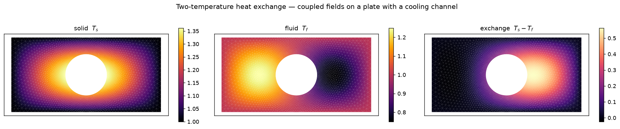
\(T_s\) and \(T_f\) are genuinely different fields; the third panel is the computed exchange \(T_s-T_f\) — the local driving force for heat transfer between the phases.
What to notice
- Complex geometry is free: shapely CSG in, a meshed
jno.domainout —box.difference(...)for the channel, a namedringrefined independently of thebulk. - Multi-field coupling is just more residual terms;
fem.problem.offsetslices the block solution back into per-field vectors. - Bring your own solver through
solve_fn(herelineax) — and the same hook accepts anoptimistixNewton (nonlinear) or adiffraxstepper (transient)..solve()'s default is only a convenience. - Verified by the method of manufactured solutions: impose a known \(T_s^\*,T_f^\*\) on the full boundary and recover it — rel-L2 \(\sim 3\times10^{-5}\), the standard correctness gate for a FEM code.
Full script
"""Coupled multiphysics on a complex domain: the two-temperature (local thermal non-equilibrium)
model on a plate with a cooling channel. Two fields share the domain -- a solid temperature ``T_s``
and a fluid temperature ``T_f`` -- exchanging heat through an interphase term ``h (T_s - T_f)``:

    -k_s lap T_s + h (T_s - T_f) = f_s
    -k_f lap T_f - h (T_s - T_f) = f_f

This shows off the FEM solver on the things that matter in practice, not a unit square:

* a real CSG domain -- ``box.difference(channel)`` (a cooling hole), authored with shapely;
* NAMED sub-regions with DIFFERENT mesh sizes -- a refined annulus ``ring`` hugs the channel
  (steep gradients) while the ``bulk`` stays coarse (``build_mesh(..., sizes={"ring": ...})``);
* genuine multi-field COUPLING -- two ``fem_symbols`` fields with a cross term, assembled as one
  block system;
* the coupled system is solved with a bring-your-own dense solver (jnp.linalg.solve);
  you never call jno's built-in solver.

Verified by the method of manufactured solutions (impose a known ``T_s*, T_f*`` on the full
boundary, recover it): a convergent rel-L2, the standard correctness gate for a FEM code.
"""

import os

os.environ["MPLBACKEND"] = "Agg"

import jax

jax.config.update("jax_enable_x64", True)  # the assembler builds in float64

from pathlib import Path  # noqa: E402

import jax.numpy as jnp  # noqa: E402
import matplotlib.pyplot as plt  # noqa: E402
import matplotlib.tri as mtri  # noqa: E402
import numpy as np  # noqa: E402
from shapely.geometry import Point, box  # noqa: E402

import jno  # noqa: E402

PI = np.pi
k_s, k_f, h = 1.0, 0.6, 8.0  # solid/fluid conductivities, interphase exchange coefficient
# manufactured fields with DISTINCT patterns (one central lobe vs two), so the coupling is visible
gs = lambda x, y: 0.40 * jno.np.sin(PI * x / 2) * jno.np.sin(PI * y)  # noqa: E731  one lobe; lap = -(5/4)pi^2 gs
gf = lambda x, y: 0.25 * jno.np.sin(PI * x) * jno.np.sin(PI * y)  # noqa: E731  two lobes; lap = -2 pi^2 gf
Ts_star = lambda x, y: 1.0 + gs(x, y)  # noqa: E731
Tf_star = lambda x, y: 1.0 + gf(x, y)  # noqa: E731
lap_Ts = lambda x, y: -(5 * PI**2 / 4) * gs(x, y)  # noqa: E731
lap_Tf = lambda x, y: -(2 * PI**2) * gf(x, y)  # noqa: E731

# complex domain: a plate with a cooling channel; refine a named annulus around the channel
channel = Point(1.0, 0.5).buffer(0.28)
ring = Point(1.0, 0.5).buffer(0.5).difference(channel).intersection(box(0, 0, 2, 1))
dom = jno.domain({"bulk": box(0, 0, 2, 1).difference(channel).difference(ring), "ring": ring})
dom = dom.build_mesh(0.06, sizes={"ring": 0.025})  # coarse bulk, fine ring

Ts, qs = dom.fem_symbols(names=("Ts", "qs"))
Tf, qf = dom.fem_symbols(names=("Tf", "qf"))
xi, yi, _ = dom.variable("interior", split=True)
xb, yb, _ = dom.variable("boundary", split=True)
s, vs, f, vf = Ts.bind(x=xi, y=yi), qs.bind(x=xi, y=yi), Tf.bind(x=xi, y=yi), qf.bind(x=xi, y=yi)

exch = Ts_star(xi, yi) - Tf_star(xi, yi)
f_s = -k_s * lap_Ts(xi, yi) + h * exch  # manufactured sources from -k lap T* +/- h (T_s* - T_f*)
f_f = -k_f * lap_Tf(xi, yi) - h * exch
fem = jno.fem(
    [
        k_s * (s.x * vs.x + s.y * vs.y) + h * (s - f) * vs - f_s * vs,  # solid energy balance
        k_f * (f.x * vf.x + f.y * vf.y) - h * (s - f) * vf - f_f * vf,  # fluid energy balance
        Ts(xb, yb) - Ts_star(xb, yb),  # manufactured Dirichlet (outer wall + channel)
        Tf(xb, yb) - Tf_star(xb, yb),
    ]
)

# bring-your-own solver: a dense direct solve (the default matrix-free Krylov is for large elliptic systems)
sol = np.asarray(fem.solve(solve_fn=lambda A, b: jnp.linalg.solve(A, b)))
off = fem.offsets  # per-field slices into the coupled solution vector
Th_s, Th_f = sol[off[0] : off[1]], sol[off[1] :]
pts = np.asarray(fem.points)
xs, ys = pts[:, 0], pts[:, 1]
ref_s = 1 + 0.40 * np.sin(PI * xs / 2) * np.sin(PI * ys)
ref_f = 1 + 0.25 * np.sin(PI * xs) * np.sin(PI * ys)
rels = float(np.linalg.norm(Th_s - ref_s) / np.linalg.norm(ref_s))
relf = float(np.linalg.norm(Th_f - ref_f) / np.linalg.norm(ref_f))
print("\nCoupled two-temperature model on a plate with a cooling channel (dense solve)")
print(f"  fields={len(off) - 1}  dofs={fem.dofs}  bulk/ring mesh = 0.06 / 0.025")  # offsets = [0, n1, n2]
print(f"  MMS recovery rel-L2:  T_s={rels:.3e}  T_f={relf:.3e}")

# ---- render the actual computed fields (no invented structure) ----
tris = np.asarray(fem.domain.built_mesh.cells_dict["triangle"])
triang = mtri.Triangulation(xs, ys, tris)
fig, ax = plt.subplots(1, 3, figsize=(16, 3.4))
panels = [
    (Th_s, "solid  $T_s$", "inferno"),
    (Th_f, "fluid  $T_f$", "inferno"),
    (Th_s - Th_f, "exchange  $T_s-T_f$", "magma"),
]
for a, (field, title, cmap) in zip(ax, panels):
    tpc = a.tripcolor(triang, field, cmap=cmap, shading="gouraud")
    a.triplot(triang, color="w", lw=0.15, alpha=0.45)  # the actual mesh: coarse bulk, fine ring
    fig.colorbar(tpc, ax=a, shrink=0.85)
    a.set_title(title, fontsize=11)
    a.set_aspect("equal")
    a.set_xticks([])
    a.set_yticks([])
fig.suptitle("Two-temperature heat exchange — coupled fields on a plate with a cooling channel", fontsize=12)
fig.tight_layout()
fig.savefig(Path(__file__).parents[2] / "assets" / "coupled_two_temperature_2d.png", dpi=130, bbox_inches="tight")

assert fem.is_linear and len(off) == 3  # 2 coupled fields -> offsets [0, n1, n1+n2]
assert rels < 2e-3 and relf < 2e-3, f"MMS recovery too loose: T_s={rels:.3e} T_f={relf:.3e}"