Stokes flow past a cylinder (complex domain, Taylor-Hood)

Download .py Back to chapter

The canonical viscous-flow benchmark on a domain with a hole. A creeping (Stokes) flow is driven through a channel obstructed by a cylinder, discretised with the inf-sup-stable Taylor-Hood pair — P2 velocity, P1 pressure — coupled in one block:

\[-\mu\,\Delta \mathbf{u} + \nabla p = 0,\qquad \nabla\!\cdot\mathbf{u} = 0.\]

Complex domain, refined at the obstacle

The channel minus a cylinder is one shapely line; a named ring around the cylinder is meshed finer than the open channel, where the velocity gradients are steep:

cyl  = Point(1.5, 0.5).buffer(0.22)
ring = Point(1.5, 0.5).buffer(0.46).difference(cyl).intersection(box(0, 0, L, H))
dom  = jno.domain({"bulk": box(0, 0, L, H).difference(cyl).difference(ring), "ring": ring})
dom  = dom.build_mesh(0.12, sizes={"ring": 0.05})   # coarse channel, fine collar

Mixed boundary data, no extra API

A parabolic profile drives the inlet and the outlet — exact for Stokes flow, which is fore-aft symmetric at \(Re=0\) — while the walls and the cylinder are no-slip. One jno.np.where on the boundary coordinate picks the driven faces; everything else is zero:

u_in = jno.np.where(xb < 1e-6, parab(yb), jno.np.where(xb > L - 1e-6, parab(yb), 0.0))
fem = jno.fem([
    mu * inner(gu, gv, n_contract=2) - pp * trace(gv),   # momentum
    -qq * trace(gu),                                      # incompressibility
    u(xb, yb)[0] - u_in,                                  # parabola at inlet/outlet, 0 on walls+cylinder
    u(xb, yb)[1] - 0.0,
    p.pin(),                                              # gauge-fix the pressure null space
])
sol = fem.solve(solve_fn=lambda A, b: lineax.linear_solve(lineax.MatrixLinearOperator(A), b).value)

The result

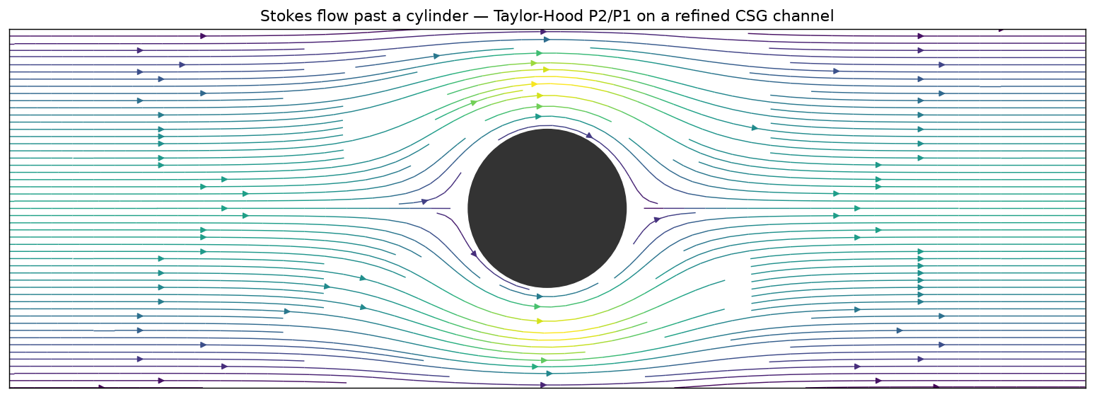
Streamlines split around the cylinder, accelerate at its flanks (colour = speed), and re-converge downstream — the textbook creeping-flow picture.

What to notice

• Complex geometry + local refinement in two lines of shapely; the ring is refined independently of the bulk.
• Taylor-Hood multiphysics: a P2 vector velocity and a P1 pressure as two fem_symbols fields, assembled as one inf-sup-stable block. fem.problem.offset slices the velocity back out.
• Bring your own solver (lineax) through solve_fn.
• Verified by a physical invariant, not an analytic solution. A centred cylinder makes Stokes flow top-bottom symmetric, so \(u_x(x,y)=u_x(x,H-y)\) and \(u_y(x,y)=-u_y(x,H-y)\); the measured symmetry error is \(\sim2\times10^{-3}\).

Full script

"""Stokes flow past a cylinder on a complex domain -- the canonical viscous-flow benchmark. A
creeping flow is driven through a channel obstructed by a cylinder, with the inf-sup-stable
Taylor-Hood pair (P2 velocity, P1 pressure) coupled in one block:

    -mu lap u + grad p = 0,   div u = 0.

* complex CSG domain -- ``box.difference(cylinder)``, with a named ``ring`` around the cylinder
  meshed finer than the rest of the channel (steep gradients hug the obstacle);
* a parabolic profile drives the inlet AND the outlet -- exact for *Stokes* flow, which is
  fore-aft symmetric (Re = 0) -- while the walls and the cylinder are no-slip;
* solved with a bring-your-own dense direct solver via `fem.solve(solve_fn=...)`.

Verified without an analytic solution by a physical invariant: a centred cylinder makes the Stokes
flow top-bottom symmetric, so the computed field must satisfy ``u_x(x, y) = u_x(x, H-y)`` and
``u_y(x, y) = -u_y(x, H-y)``. We measure the residual symmetry error on a regular grid.
"""

import os

os.environ["MPLBACKEND"] = "Agg"
os.environ["FEAX_X64"] = "1"  # float64 feax assembly (the test session defaults FEAX_X64=0; this subprocess opts in)

import jax

jax.config.update("jax_enable_x64", True)  # the assembler builds in float64

from pathlib import Path  # noqa: E402

import jax.numpy as jnp  # noqa: E402
import matplotlib.pyplot as plt  # noqa: E402
import numpy as np  # noqa: E402
from scipy.interpolate import griddata  # noqa: E402
from shapely.geometry import Point, box  # noqa: E402

import jno  # noqa: E402

mu, L, H = 1.0, 3.0, 1.0
inner, grad, trace = jno.np.inner, jno.np.grad, jno.np.trace
parab = lambda y: 4.0 * y * (H - y)  # noqa: E731  Poiseuille inflow/outflow profile, peak 1

# complex domain: a channel obstructed by a centred cylinder; refine a named ring around it
cyl = Point(1.5, 0.5).buffer(0.22)
ring = Point(1.5, 0.5).buffer(0.46).difference(cyl).intersection(box(0, 0, L, H))
dom = jno.domain({"bulk": box(0, 0, L, H).difference(cyl).difference(ring), "ring": ring})
dom = dom.build_mesh(0.12, sizes={"ring": 0.05})  # coarse channel, fine collar at the cylinder

u, v = dom.fem_symbols(value_shape=(2,), names=("u", "v"), order=2)  # P2 velocity
p, q = dom.fem_symbols(names=("p", "q"), order=1)  # P1 pressure
xi, yi, _ = dom.variable("interior", split=True)
xb, yb, _ = dom.variable("boundary", split=True)
gu, gv = grad(u, [xi, yi]), grad(v, [xi, yi])
pp, qq = p.bind(x=xi, y=yi), q.bind(x=xi, y=yi)

# inlet & outlet get the parabolic profile; walls and cylinder are no-slip (0)
u_in = jno.np.where(xb < 1e-6, parab(yb), jno.np.where(xb > L - 1e-6, parab(yb), 0.0))
fem = jno.fem(
    [
        mu * inner(gu, gv, n_contract=2) - pp * trace(gv),  # momentum (no body force)
        -qq * trace(gu),  # incompressibility
        u(xb, yb)[0] - u_in,  # x-velocity: parabola at inlet/outlet, 0 on walls + cylinder
        u(xb, yb)[1] - 0.0,  # y-velocity: 0 everywhere on the boundary
        p.pin(),  # gauge-fix: remove the pressure null space
    ]
)

# bring-your-own solver: a dense direct solve (the default matrix-free Krylov is for large elliptic systems)
sol = np.asarray(fem.solve(solve_fn=lambda A, b: jnp.linalg.solve(A, b)))
off = fem.offsets
uu = sol[off[0] : off[1]].reshape(-1, 2)  # velocity (n_vel_nodes, 2)
pts_v = np.asarray(fem.field_points[0])

# regular grid (mask the cylinder), used for both the symmetry gate and the figure
gx, gy = np.meshgrid(np.linspace(0, L, 300), np.linspace(0, H, 100))
inside = np.hypot(gx - 1.5, gy - 0.5) > 0.22
UX = np.where(inside, griddata(pts_v, uu[:, 0], (gx, gy), method="linear"), np.nan)
UY = np.where(inside, griddata(pts_v, uu[:, 1], (gx, gy), method="linear"), np.nan)
m = np.isfinite(UX) & np.isfinite(UX[::-1])  # nodes whose mirror is also valid
sym = float(np.linalg.norm(np.r_[(UX - UX[::-1])[m], (UY + UY[::-1])[m]]) / np.linalg.norm(np.r_[UX[m], UY[m]]))
print("\nStokes flow past a cylinder (Taylor-Hood P2/P1, dense solve)")
print(f"  fields={len(off) - 1}  dofs={fem.dofs}  channel/ring mesh = 0.12 / 0.05")  # offsets = [0, n_v, n_v+n_p]
print(f"  top-bottom symmetry error (should be ~0): {sym:.3e}")

# ---- render the actual computed flow (streamlines squeezing past the obstacle) ----
speed = np.hypot(UX, UY)
fig, ax = plt.subplots(figsize=(13, 4.4))
ax.streamplot(gx, gy, UX, UY, color=speed, cmap="viridis", density=1.7, linewidth=0.8)
ax.add_patch(plt.Circle((1.5, 0.5), 0.22, color="0.2"))
ax.set_aspect("equal")
ax.set_xlim(0, L)
ax.set_ylim(0, H)
ax.set_xticks([])
ax.set_yticks([])
ax.set_title("Stokes flow past a cylinder — Taylor-Hood P2/P1 on a refined CSG channel", fontsize=12)
fig.tight_layout()
fig.savefig(Path(__file__).parents[2] / "assets" / "stokes_flow_around_cylinder.png", dpi=130, bbox_inches="tight")

assert len(off) == 3 and sym < 2e-2, f"Stokes flow not top-bottom symmetric: {sym:.3e}"  # [0, n_v, n_v+n_p]