Poroelastic Consolidation (Biot)

Download .py Back to chapter

Load a water-saturated soil column and it does not settle all at once: the pore water carries the load instantly (an excess-pressure spike), then slowly drains out the top while the grains take over and the column consolidates. This is Biot poroelasticity — solid displacement u and pore pressure p two-way coupled, in one jno.fem:

\[ \nabla\!\cdot\sigma' - \alpha\,\nabla p = 0,\quad \sigma' = \lambda\,\mathrm{tr}(\varepsilon)I + 2\mu\,\varepsilon;\qquad S\,\partial_t p + \alpha\,\partial_t(\nabla\!\cdot u) = \kappa\,\nabla^2 p . \]

The Biot coupling is a cross-field mass term

-alpha*pb*trace(ev) feeds pressure into the solid balance; the fluid balance is fed back by the rate of volume change alpha*(div u)_t. Written naively that needs a mixed space–time derivative, so it is integrated by parts in space to -alpha*(u_t . grad q) — only first-order derivatives, and it lands in the mass matrix as a cross-field (p–u) block, which is the Biot coupling:

u, phi = d.fem_symbols(value_shape=(2,), names=("u", "phi"), order=2)   # displacement (P2)
p, q   = d.fem_symbols(names=("p", "q"), order=1)                       # pore pressure (P1)
eu, ev = symgrad(u, [xi, yi]), symgrad(phi, [xi, yi])

solid = lam*trace(eu)*trace(ev) + 2*mu*inner(eu, ev, n_contract=2) - alpha*pb*trace(ev)
fluid = S*pb.t*qb - alpha*(ub.t[0]*qb.x + ub.t[1]*qb.y) + kappa*(pb.x*qb.x + pb.y*qb.y)
fem   = jno.fem([solid, fluid, traction, p(xt,yt) - 0.0, u(xbo,ybo)[1] - 0.0, u(xl,yl)[0] - 0.0, ...])

The boundary conditions make it a 1-D consolidation test: drained top (p = 0) under a load, an impermeable roller base, and confined (roller) sides.

Linear ⇒ factor once; the load lives in the forcing vector

The system is linear with a constant operator, so factor M + dt·A once and back-substitute each step. The constant top load comes from fem.operator.forcing_vector_fn (a transient problem keeps its load there, not in the weak-form residual):

M, A = _csc(fem.M), _csc(fem.operator.A)
b    = fem.operator.forcing_vector_fn(0.0, {})       # constant top-load vector
lu   = splu((M + dt*A).tocsc())                      # factor ONCE
for step in range(nsteps):
    w = lu.solve(M @ w + dt*b)                        # back-substitute

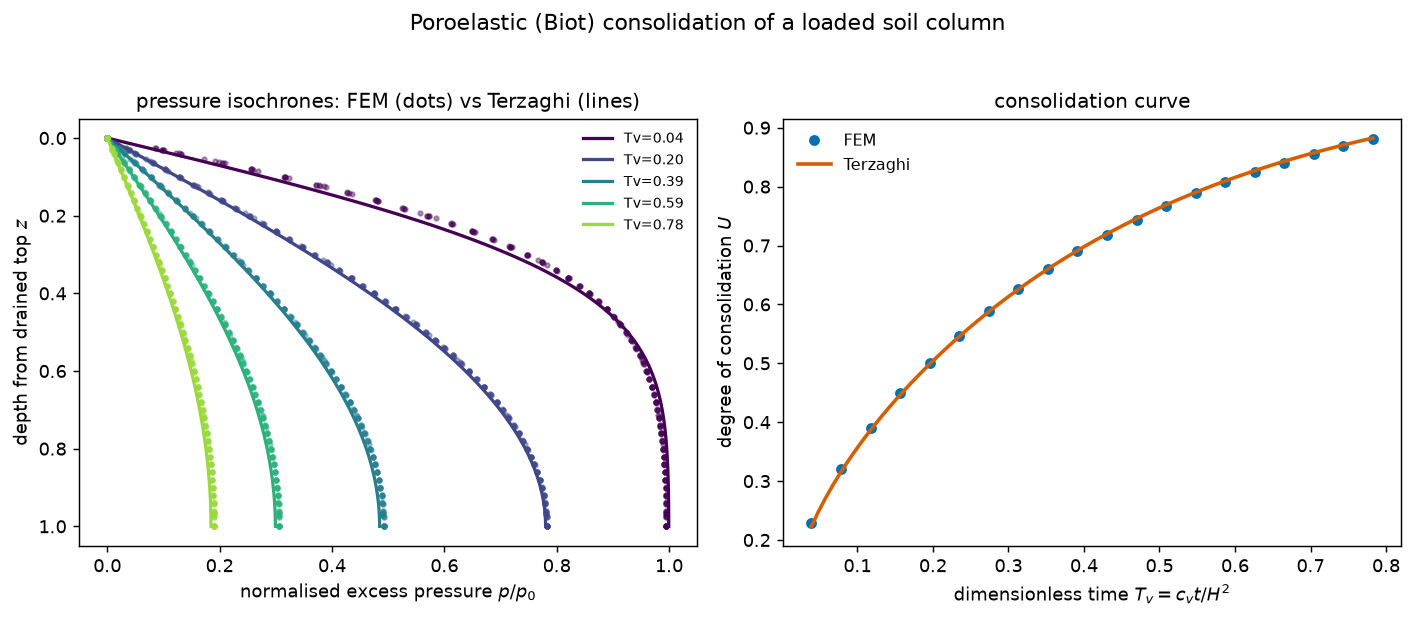
Validated against Terzaghi to ~0.5 %

The computed pressure isochrones fall right on the classic Terzaghi curves at every dimensionless time \(T_v = c_v t / H^2\), and the degree of consolidation \(U(T_v)\) matches the analytic series to within 0.5 % (right panel above). The excess pressure dissipates monotonically and the column keeps settling as the water drains — exactly the consolidation story. The animation shows the computed pore pressure on the computed (settling) mesh; nothing is painted in.

References: K. von Terzaghi, Erdbaumechanik (1925) — 1-D consolidation; M. A. Biot, J. Appl. Phys. 12:155 (1941) — three-dimensional consolidation.