Conduction + Grey-Body Enclosure Radiation (concentric cylinders)

Download .py Back to chapter

Two solid rings separated by a vacuum gap: heat conducts from the hot inner edge through the inner ring, radiates across the gap to the outer ring, then conducts out to the cold edge. Radiation is nonlinear (\(T^4\)) and nonlocal — every gap-facing element exchanges with every other through the view-factor matrix — so it cannot be a local weak term. jNO supplies the view matrix; you write the grey-body radiosity as math in jno.np and couple it to the conduction FEM as a consistent surface load. There is no jno.radiation() helper.

The view matrix is a first-class object

domain.enclosure(tags) discretises the radiating surfaces into mesh-aligned elements and returns a quality-gated view factor — fully geometry-determined, so a concave surface keeps its self-view (\(F_{22}=1-r_1/r_2\) for the outer cylinder):

gap = d.enclosure(["inner_gap", "outer_gap"])   # name the surfaces once (axisymmetric=True for r,z)
gap.check()                                      # closure (Σ_j F_ij→1) + reciprocity (A_i F_ij = A_j F_ji)
F   = gap.view_factor
eps = gap.emissivity({"inner_gap": 0.8, "outer_gap": 0.6})
rho = 1.0 - eps

You write the radiosity; it stays traced

def q_rad(u):                        # net flux per element:  q = σ·G·T⁴, G=(I−F)(I−ρF)⁻¹diag(ε)
    Ts = gap.field(u)                # nonlocal gather: per-element temperature from the solution
    J  = jno.np.linalg.solve(jno.np.eye(gap.size) - rho[:, None] * F, eps * SIGMA * (Ts + KELVIN)**4)
    return J - F @ J

gap.field(u) gathers the per-element temperature; gap.load(q) scatters a per-element flux back to the FEM nodes as the consistent surface load \(\int_\Gamma q\,v\,ds\). Because the radiosity is jno.np, a trainable jno.np.parameter emissivity flows through it for inverse problems.

Couple and solve

The radiation BC \(-k\,\partial T/\partial n = q_{rad}\) enters the residual as a load, so you solve \(A u = b - \texttt{gap.load}(q_{rad}(u))\). jNO imposes no solver; the Dirichlet conditions are penalty-enforced (so \(A\) is ill-conditioned) — a direct linear solve handles it (a matrix-free iterative solver may stall). The whole thing stays jax-native and differentiable with a short direct-solve Newton (jax.lax.custom_root for implicit diff), so jax.grad/crux recover an emissivity through the radiation:

A = fem.operator[0].todense()        # BCOO → dense via the jax path (.todense() is fast; np.asarray is NOT)
b = fem.operator[1]

def newton(residual, u0, steps=50, tol=1e-9):       # BYO; ~10 lines, no external solver
    f = lambda u: jnp.asarray(residual(u)).reshape(-1)
    def stepper(fn, x0):
        def body(s):
            du = jnp.linalg.solve(jax.jacfwd(fn)(s[0]), -fn(s[0]))   # DIRECT inner solve each step
            return s[0] + du, jnp.linalg.norm(du), s[2] + 1
        return jax.lax.while_loop(lambda s: (s[1] > tol) & (s[2] < steps), body, (x0, 1.0, 0))[0]
    tangent = lambda g, y: jnp.linalg.solve(jax.jacfwd(g)(jnp.zeros_like(y)), y)
    return jax.lax.custom_root(f, jnp.asarray(u0).reshape(-1), stepper, tangent)

T = newton(lambda u: A @ u - b + gap.load(q_rad(u)), jnp.linalg.solve(A, b))

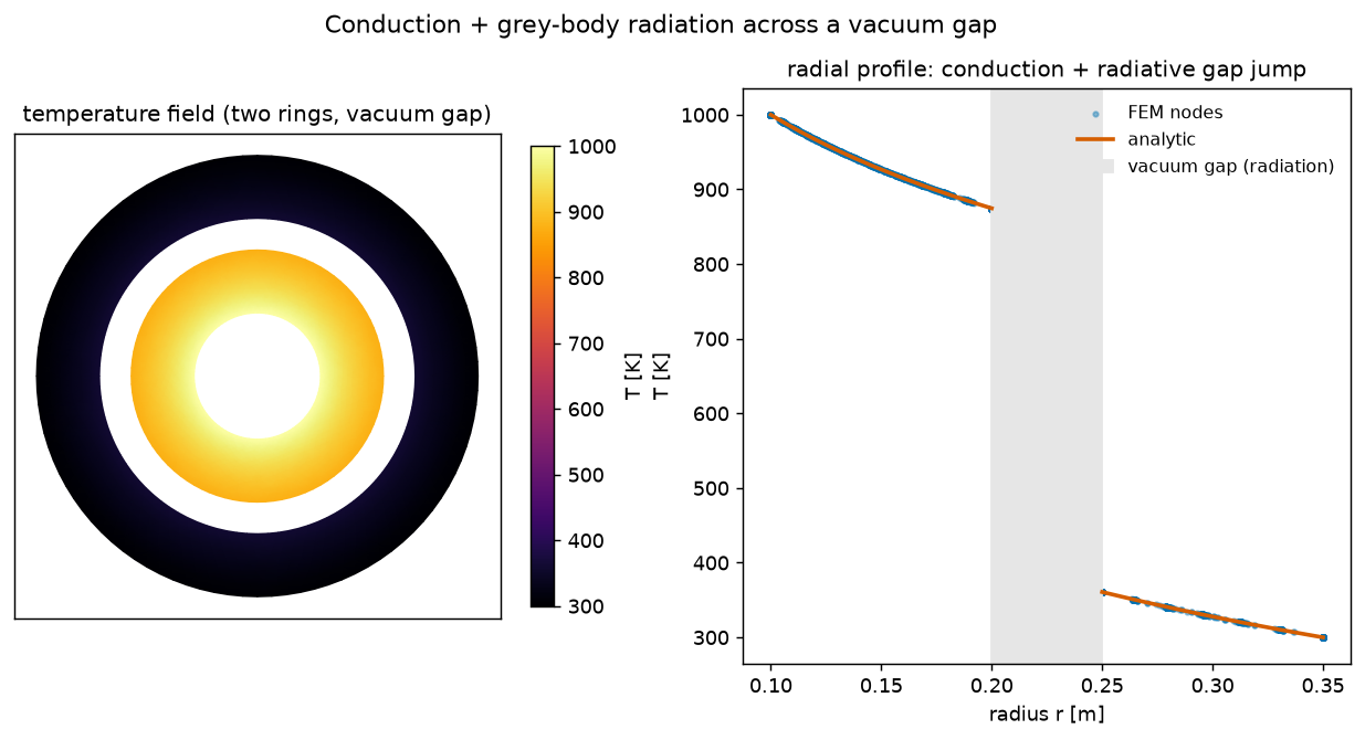
It matches the closed form

The coupled surface temperatures and heat flow reproduce the analytic two-surface series \(Q = 2\pi r_1\sigma(T_{s1}^4-T_{s2}^4)/(1/\varepsilon_1+(r_1/r_2)(1/\varepsilon_2-1))\) to under 1 % (Ts1 874.7 K, Ts2 360.6 K). The radial-profile panel shows the logarithmic conduction profile in each ring and the radiative temperature jump across the gap.

Reference: M. F. Modest, Radiative Heat Transfer, 3rd ed., Ch. 4–5 (view factors; the net-radiation / radiosity method for diffuse-grey enclosures).