Inverse problem on a complex domain (FEM tomography)

Download .py Back to chapter

The differentiable-FEM story meets the complex-geometry one. On an L-shaped part we recover a hidden conductivity field \(k(x)\) — a buried high-conductivity inclusion — from the measured response to a known source, by differentiating the FEM solve end to end:

\[\text{forward: } -\nabla\!\cdot(k(x)\,\nabla u) = f,\quad u|_{\partial\Omega}=0,\qquad \text{unknown } k(x)>0.\]

The whole inverse problem, in a few lines

k = jno.np.parameter(phi) is a trainable P1 field on the trial space. fem.solve() is the differentiable forward solve, and crux.solve minimises the data misfit plus an H1 smoothness prior (field inversion is ill-posed without one):

d = jno.domain([[0,0],[2,0],[2,1],[1,1],[1,2],[0,2]]).build_mesh(0.06)   # L-shape, not a square
...
k   = jno.np.parameter(phi, name="k")
fem = jno.fem([k * (ui.x*vi.x + ui.y*vi.y) - f*vi, u(xb, yb) - 0.0])
k.initialize(jax.nn.initializers.constant(1.0))                          # start from a flat guess
k.optimizer(optax.adam(2e-2))
crux = jno.core([(fem.solve() - u_obs).mse, 2e-3 * k.regularize("h1seminorm").mean], domain=...)
crux.solve(700)                                                          # gradients flow through the solve

The synthetic data u_obs comes from the same assembly evaluated at the true field — fem.operator.evaluate({"k": k_true}) — so there is one weak form for both the forward and the inverse direction.

The result

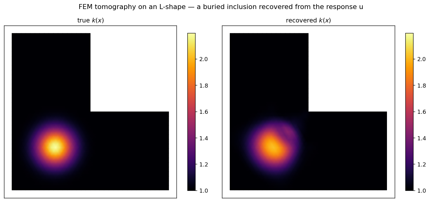
The reconstruction recovers the buried inclusion at the right place with nearly the right peak (\(\sim\)2.0 vs 2.2) — rel-L2 \(\sim2.5\times10^{-2}\).

What to notice

• The complex domain changes nothing about the workflow: the L-shape is one vertex list; the inverse machinery is identical to a square.
• fem.solve() is differentiable — crux.solve backpropagates the data misfit through the linear FEM solve to every nodal value of k(x).
• Field inversion needs a prior: k.regularize("h1seminorm") keeps the ill-posed reconstruction smooth; without it the recovered field is dominated by noise.
• The same pattern recovers a scalar parameter (drop the field, use jno.np.parameter((1,))) or a transient coefficient (assemble with time=... and train through the trajectory).

Full script

"""Inverse problem on a complex domain: recover a buried conductivity field through a differentiable
FEM solve. On an L-shaped part,

    forward:  -div(k(x) grad u) = f,   u = 0 on the boundary,   with unknown k(x) > 0,

we measure the response ``u`` to a known source and reconstruct the entire nodal field ``k(x)`` --
a hidden high-conductivity inclusion buried in the part. This is FEM tomography / parameter-field
identification, and it ties the differentiable-FEM story to the complex-geometry one:

* the domain is a non-convex L-shape (a vertex list -> ``jno.domain(...)``), not a square;
* ``k = jno.np.parameter(phi)`` is a trainable P1 field on the trial space;
* ``fem.solve()`` is the differentiable forward solve, and ``crux.solve`` minimises the data misfit
  plus an H1-seminorm smoothness prior (field inversion is ill-posed without one).
"""

import os

os.environ["MPLBACKEND"] = "Agg"

import jax

jax.config.update("jax_enable_x64", True)  # the assembler builds in float64

from pathlib import Path  # noqa: E402

import jax.numpy as jnp  # noqa: E402
import matplotlib.pyplot as plt  # noqa: E402
import matplotlib.tri as mtri  # noqa: E402
import numpy as np  # noqa: E402
import optax  # noqa: E402

import jno  # noqa: E402

# complex domain: an L-shaped part (re-entrant corner), from a vertex list
d = jno.domain([[0, 0], [2, 0], [2, 1], [1, 1], [1, 2], [0, 2]]).build_mesh(0.06)
u, phi = d.fem_symbols()
xi, yi, _ = d.variable("interior", split=True)
xb, yb, _ = d.variable("boundary", split=True)
ui, vi = u.bind(x=xi, y=yi), phi.bind(x=xi, y=yi)
f = 40.0 * (jno.np.sin(np.pi * xi / 2) + jno.np.sin(np.pi * yi / 2))  # strong source -> u sensitive to k

nodes = np.asarray(d.built_mesh.points)[:, :2]
k_true = 1.0 + 1.2 * np.exp(-((nodes[:, 0] - 0.55) ** 2 + (nodes[:, 1] - 0.55) ** 2) / (2 * 0.16**2))  # buried inclusion

# one parametric assembly: synthesise full-field data at the true k ...
k = jno.np.parameter(phi, name="k")
fem = jno.fem([k * (ui.x * vi.x + ui.y * vi.y) - f * vi, u(xb, yb) - 0.0], quad_degree=3)
A_true, b = fem.operator.evaluate({"k": jnp.asarray(k_true)})
u_obs = jnp.linalg.solve(jnp.asarray(A_true), jnp.asarray(b).reshape(-1))

# ... then recover k(x) from u_obs through the differentiable solve + an H1 smoothness prior
k.dtype(jnp.float64)
k.initialize(jax.nn.initializers.constant(1.0))  # start from a uniform field
k.optimizer(optax.adam(2e-2))
crux = jno.core(
    [(fem.solve() - u_obs).mse, 2e-3 * k.regularize("h1seminorm").mean],
    domain=jno.domain.from_array({"_": np.zeros((1, 1))}),
)
crux.solve(700)

rec = np.asarray(crux.eval([k])).reshape(-1)  # the recovered nodal field (do NOT index [0])
rel = float(np.linalg.norm(rec - k_true) / np.linalg.norm(k_true))
print("\nInverse conductivity on an L-shaped domain (differentiable FEM + crux)")
print(f"  nodes={k_true.shape[0]}  k(x) rel-L2={rel:.3e}  peak rec/true={rec.max():.3f}/{k_true.max():.3f}")

# ---- render true vs recovered field (the actual crux output, no invented structure) ----
tris = np.asarray(d.built_mesh.cells_dict["triangle"])
triang = mtri.Triangulation(nodes[:, 0], nodes[:, 1], tris)
vmax = float(max(k_true.max(), rec.max()))
fig, ax = plt.subplots(1, 2, figsize=(11, 5.2))
for a, field, title in ((ax[0], k_true, "true $k(x)$"), (ax[1], rec, "recovered $k(x)$")):
    tpc = a.tripcolor(triang, field, cmap="inferno", shading="gouraud", vmin=1.0, vmax=vmax)
    fig.colorbar(tpc, ax=a, shrink=0.85)
    a.set_aspect("equal")
    a.set_xticks([])
    a.set_yticks([])
    a.set_title(title, fontsize=11)
fig.suptitle("FEM tomography on an L-shape — a buried inclusion recovered from the response u", fontsize=12)
fig.tight_layout()
fig.savefig(Path(__file__).parents[2] / "assets" / "inverse_conductivity_lshape.png", dpi=130, bbox_inches="tight")

assert rel < 0.1, f"inclusion not recovered: rel-L2 {rel:.3e}"