Kovasznay Flow (steady Navier–Stokes)

Download .py Back to chapter

Kovasznay (1948) found a rare closed-form solution of the full nonlinear incompressible Navier–Stokes equations — the laminar wake behind a 2-D grid — which makes it the canonical verification problem for an incompressible flow solver: there is an exact field to compare against. At \(Re=1/\nu=40\),

\[u = 1 - e^{\lambda x}\cos 2\pi y,\quad v = \tfrac{\lambda}{2\pi}e^{\lambda x}\sin 2\pi y,\quad p = \tfrac12(1-e^{2\lambda x}),\quad \lambda = \tfrac{Re}{2}-\sqrt{\tfrac{Re^2}{4}+4\pi^2}.\]

The weak form

The convective term \((\mathbf{u}\cdot\nabla)\mathbf{u}\) — the unknown contracted with itself — makes the form nonlinear, so jno.fem returns a coupled residual operator with an autodiff Jacobian, solved by Newton on the inf–sup-stable Taylor–Hood pair (P2 velocity / P1 pressure):

conv = inner(gu, ub, n_contract=1)  # (u.grad) u
momentum = inner(conv, vv, n_contract=1) + nu * inner(gu, gv, n_contract=2) - pp * trace(gv)
fem = jno.fem([momentum, -qq * trace(gu),
               u(xb, yb)[0] - bx, u(xb, yb)[1] - by,   # analytic velocity on the boundary
               p.pin(p0)])                              # gauge-fix pressure to the analytic value p0

Computed Kovasznay speed and streamlines, the laminar wake behind a grid.

What to notice

The convective nonlinearity routes the whole system to the nonlinear coupled operator; the Jacobian is autodiffed and Newton converges from rest.
The recovered velocity matches the analytic Kovasznay field to relative \(L^2 \approx 8\times10^{-5}\) — the order of accuracy of this solve is certified in tests/test_fem_convergence.py.

Full script

"""Kovasznay flow -- a closed-form steady Navier-Stokes benchmark via ``jno.fem``.

    (u.grad)u - nu lap u + grad p = 0,   div u = 0,   Re = 1/nu = 40.

Kovasznay (1948) found a rare *exact* solution of the full nonlinear, incompressible Navier-Stokes
equations -- the laminar wake behind a 2D grid:

    u = 1 - e^{lam x} cos(2 pi y),  v = (lam/2pi) e^{lam x} sin(2 pi y),  p = (1 - e^{2 lam x})/2,
    lam = Re/2 - sqrt(Re^2/4 + 4 pi^2).

This makes it the canonical *verification* problem for an incompressible NS solver: there is a true
field to compare against. The convective term ``(u.grad)u`` -- the unknown contracted with itself --
is a genuine nonlinearity, so ``jno.fem`` routes the inf-sup-stable Taylor-Hood (P2 velocity / P1
pressure) system to its coupled nonlinear operator and the Jacobian comes from autodiff. We solve it
with a Newton root-find from rest, and check the recovered velocity against the analytic field.

Reference: L. I. G. Kovasznay, "Laminar flow behind a two-dimensional grid", Proc. Camb. Phil. Soc.
44(1), 58-62 (1948).
"""

import os

os.environ["MPLBACKEND"] = "Agg"

import jax

jax.config.update("jax_enable_x64", True)  # the assembler builds in float64

from pathlib import Path  # noqa: E402

import matplotlib.pyplot as plt  # noqa: E402
import numpy as np  # noqa: E402
from scipy.interpolate import griddata  # noqa: E402
from shapely.geometry import box  # noqa: E402

import jno  # noqa: E402

inner, grad, trace = jno.np.inner, jno.np.grad, jno.np.trace
dense = lambda A: np.asarray(A.todense()) if hasattr(A, "todense") else np.asarray(A)  # noqa: E731

nu = 0.025  # Re = 1/nu = 40
Re = 1.0 / nu
lam = Re / 2 - np.sqrt(Re**2 / 4 + 4 * np.pi**2)
ue = lambda x, y: 1.0 - np.exp(lam * x) * np.cos(2 * np.pi * y)  # noqa: E731  analytic velocity
ve = lambda x, y: lam / (2 * np.pi) * np.exp(lam * x) * np.sin(2 * np.pi * y)  # noqa: E731
pe = lambda x, y: 0.5 * (1.0 - np.exp(2 * lam * x))  # noqa: E731

x0, y0 = -0.5, -0.5  # the channel [-0.5, 1] x [-0.5, 1.5]
d = jno.domain(box(x0, y0, 1.0, 1.5), mesh_size=0.08)
u, v = d.fem_symbols(value_shape=(2,), names=("u", "v"), order=2)  # P2 velocity
p, q = d.fem_symbols(names=("p", "q"), order=1)  # P1 pressure (inf-sup stable)
xi, yi, _ = d.variable("interior", split=True)
xb, yb, _ = d.variable("boundary", split=True)
ub = u.bind(x=xi, y=yi)
gu, gv = grad(u, [xi, yi]), grad(v, [xi, yi])
pp, qq, vv = p.bind(x=xi, y=yi), q.bind(x=xi, y=yi), v.bind(x=xi, y=yi)
conv = inner(gu, ub, n_contract=1)  # (u.grad)u -- the convective nonlinearity
momentum = inner(conv, vv, n_contract=1) + nu * inner(gu, gv, n_contract=2) - pp * trace(gv)
bx = 1.0 - jno.np.exp(lam * xb) * jno.np.cos(2 * np.pi * yb)  # analytic velocity on the boundary
by = lam / (2 * np.pi) * jno.np.exp(lam * xb) * jno.np.sin(2 * np.pi * yb)
fem = jno.fem(
    [
        momentum,
        -qq * trace(gu),  # incompressibility
        u(xb, yb)[0] - bx,  # Dirichlet velocity = the analytic field
        u(xb, yb)[1] - by,
        p.pin(float(pe(x0, y0))),  # gauge-fix to the analytic value (min-corner) so recovered p == p* exactly
    ]
)
assert not fem.is_linear and not fem.is_transient, "Kovasznay is a steady nonlinear system"

# Newton from rest on the assembled residual / autodiff Jacobian (direct linear solve per step)
w = np.zeros(fem.dofs)
for _ in range(15):
    G = np.asarray(fem.residual(w))
    dw = np.linalg.solve(dense(fem.jacobian(w)), -G)
    w = w + dw
    if float(np.linalg.norm(dw)) < 1e-10:
        break
resid = float(np.linalg.norm(np.asarray(fem.residual(w))))
off = fem.offsets
pts_v = np.asarray(fem.field_points[0])
uu = w[off[0] : off[1]].reshape(-1, 2)
u_ex = np.stack([ue(pts_v[:, 0], pts_v[:, 1]), ve(pts_v[:, 0], pts_v[:, 1])], axis=-1)
rel = float(np.linalg.norm(uu - u_ex) / np.linalg.norm(u_ex))
print("\nKovasznay flow (steady Navier-Stokes, Taylor-Hood P2/P1)")
print(f"  Re={Re:.0f}  dofs={fem.dofs}  Newton |residual|={resid:.1e}")
print(f"  recovered velocity vs analytic Kovasznay field: rel-L2 = {rel:.2e}")

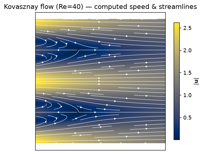
# ---- render the computed flow: speed + streamlines (the actual FEM solution) ----
gx, gy = np.meshgrid(np.linspace(x0, 1.0, 220), np.linspace(y0, 1.5, 220))
GU = griddata(pts_v, uu[:, 0], (gx, gy), method="cubic")
GV = griddata(pts_v, uu[:, 1], (gx, gy), method="cubic")
fig, ax = plt.subplots(figsize=(5.4, 4.6))
im = ax.imshow(np.hypot(GU, GV), origin="lower", extent=(x0, 1.0, y0, 1.5), cmap="cividis", aspect="auto")
ax.streamplot(gx, gy, GU, GV, color="white", density=1.1, linewidth=0.6, arrowsize=0.7)
fig.colorbar(im, ax=ax, shrink=0.85, label=r"$|\mathbf{u}|$")
ax.set_title(f"Kovasznay flow (Re={Re:.0f}) — computed speed & streamlines")
ax.set_xticks([])
ax.set_yticks([])
fig.savefig(Path(__file__).parents[2] / "assets" / "kovasznay_flow_2d.png", dpi=130, bbox_inches="tight")

assert resid < 1e-7 and rel < 1e-3, f"Kovasznay velocity not recovered: rel-L2 {rel:.2e}, residual {resid:.1e}"